Commodity-driven macroeconomic fluctuations: Does size matter?

Abstract
Commodities play a central yet often underappreciated role in shaping macroeconomic fluctuations across both advanced economies (AEs) and emerging markets and developing economies (EMDEs). This paper examines how interlinkages between the commodity sector and other sectors of the economy, both up-and downstream, condition the transmission of commodity price shocks to consumption. Rather than focusing only on sectoral size, like most of the literature, we emphasize production linkages as measured by the network-adjusted value-added share (NAVAS) of the commodity sector – or the share of the commodity sector’s value added allocated to its factor of production, directly and indirectly via the value-chain. Using panel local projections for OECD countries, we show that greater interconnectedness amplifies the positive effects of terms-of-trade gains on consumption. To interpret this result, we develop a small-open-economy model with production networks. The model highlights how the commodity sector’s interconnectedness strengthens wealth effects but dampens income effects, shaping the overall macroeconomic response. Our findings underscore the importance of network structures in explaining commodity shock propagation to consumption and welfare.

Introduction: The Reach of the Commodity Sector Matters More than its Size

Commodities play a central yet often underappreciated role in shaping macroeconomic fluctuations across both advanced economies (AEs) and emerging market and developing economies (EMDEs), with the latter generally experiencing larger macroeconomic volatility. In today’s context of climate-related supply shocks and geopolitical and trade tensions, understanding the macroeconomic impact of commodity price fluctuations is more important than ever. And this requires looking beyond the sheer size of the commodity sector and instead examining how connected the commodity sector is to the rest of the economy (Baqaee and Farhi, 2019; Bigio and La’O, 2020; Silva, 2024; Silva and others, 2024; Romero, 2025; Qiu and others, 2025). For example, the Norwegian energy sector is significantly more interconnected – as buyer and supplier of intermediates domestically – than the energy sector in Vietnam’s, despite its similar size. These interlinkages shape the reallocation of labor and capital across sectors in response to a commodity price movement and play a critical role in driving fluctuations in real activity, especially fluctuations in consumption, which is crucial for welfare.

The research summarized in this Policy Brief seeks to answer two questions: (1) How do commodity sectors’ linkages with the broader economy differ between EMDEs and AEs, and (2) How do these differences affect the propagation of commodity price shocks to the rest of the economy?

Size and Interconnectedness of the Commodity Sector in AEs and EMDEs

To assess the relative importance of size and interconnectedness of the commodity sector in explaining macroeconomic fluctuations, we compile information on consumption, output, as well as the structure of the value-chain (via input-output tables) for a panel of countries comprising both AEs and EMDEs.

Our dataset is an unbalanced annual panel comprising 66 countries, with 37 countries in the AEs group and 29 in the EMDEs group, following the IMF taxonomy. The sample spans the period from 1990 to 2018 (extended through 2023 when data availability permits) and includes country-level terms-of-trade data from the IMF’s Commodity Terms of Trade (CTOT) database, macroeconomic variables from Müller and others (2025), and the OECD’s 2018 input-output (IO) tables that capture the interlinkages of the commodity sector with the broader domestic economy.

To measure the commodity sector’s interconnectedness, we rely on the network-adjusted value-added share (NAVAS) of the commodity sector (Silva and others, 2024; Qiu and others, 2025), or the share of the commodity sector’s value added allocated to its factors of production – directly and indirectly –when considering all interlinkages, upstream and downstream.

To fix ideas, consider the following simple economy with three sectors: C (the commodity sector), A, and B, with factor shares a’ = (0.3, 0.3, 0.6). To find the NAVAS of the commodity sector, we need information on both the value-added (VA) shares (or factor shares) of each sector in the economy and the Input-Output (IO) table. If sector C does not use any input from sectors A and B, then its NAVAS is equivalent to its VA share (0.3), or the share of VA spent on production factors capital and labor.

But this is unrealistic in a modern economy where production happens along complex supply chains; IO relationships need to be considered. For example, an increase in copper prices encourages mining and extraction activities in countries that produce copper. This typically results in greater demand for industrial machinery, construction, transportation, and even financial services, all inputs to the copper industry, which itself is an input to many other domestic industries. Ultimately, allowing for all the interaction up and downstream, results in a NAVAS for the commodity sector that is higher than its VA share, as the former also accounts for all the factors bought indirectly when purchasing intermediates from the other sectors in the economy (see Gomez-Gonzalez and others, 2025 and the October 2025 Commodity Special Feature of the IMF World Economic Outlook for more details on the calculations.)

Figure 1 shows the distribution of size – measured by Domar weights – and NAVAS for the commodity sector in AEs and EMDEs in 2018.

Figure 1. Size and NAVAS across country groups

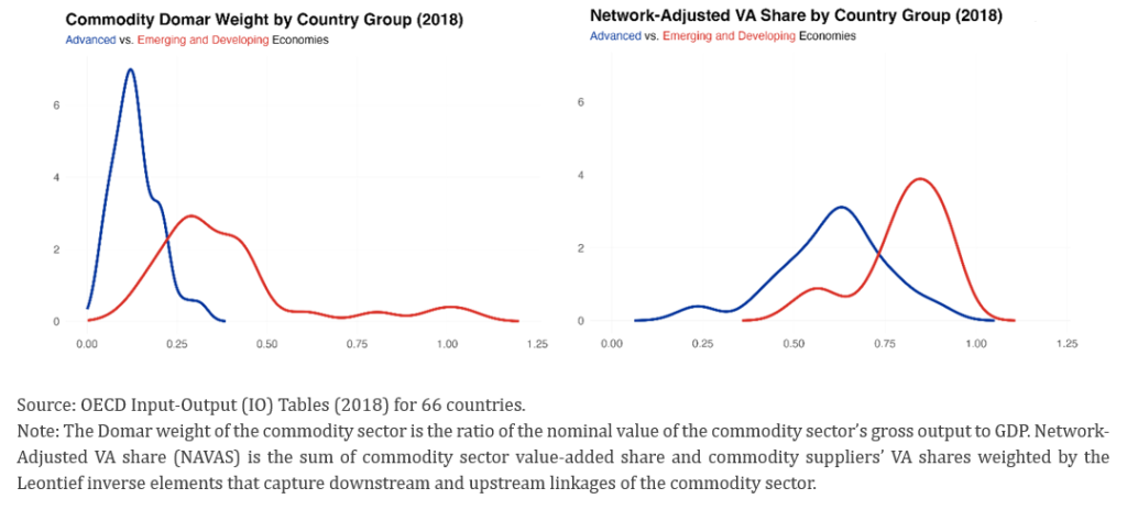
Armed with the NAVAS data for all countries in our sample, we highlight a number of stylized facts. First, the average size of the commodity sector is three times larger (Domar weight) in EMDEs than in AEs (Figure 1, panel 1), but its NAVAS is only 31 percent higher. Second, there is a lot of variation at the sectoral level: the average size is twice as large for metals, three times as large for energy and almost four times as large for agriculture compared to AEs. Third, there is also a large overlap between the right tail of the distribution of the NAVAS in AEs and the left tail in EMDEs (Figure 1, panel 2), meaning that commodity sectors in many AEs are more interconnected than in EMDEs.

Understanding Consumption Patterns Depends on Commodity Sector Interconnectedness, Beyond Size

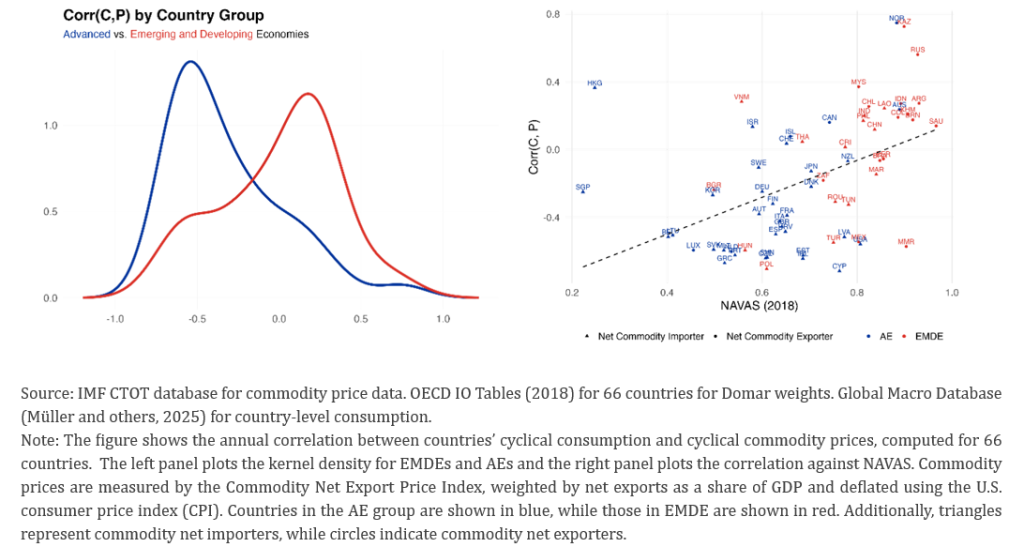
So which matters more for consumption: NAVAS or size? Figure 2, panel 1 plots the kernel distributions of the correlation between cyclical consumption and commodity prices for EMDEs and AEs. While a priori both size and NAVAS could drive such correlations, the shape of the distributions and the overlap between both groups of countries mirror the NAVAS distributions (Figure 1, panel 2) more closely than the country group distributions of Domar weights (Figure 1, panel 1). The latter are more disjoint and show a larger density around low Domar weights for AEs that would imply ceteris paribus much smaller correlation between commodity prices and consumption than shown on Figure 2, panel 1.

Another, more direct, way to look at the relationship between NAVAS and consumption is to show the relationship between the NAVAS (horizontal axis) and the correlation between countries’ cyclical consumption and commodities’ terms of trade (CTOT) (Figure 2, panel 2). The relationship is clearly positive, meaning that countries with a more interconnected commodity sector (higher NAVAS) tend to display stronger correlation between aggregate consumption and commodities terms of trade. While most EMDEs (in red) tend to be on the upper-right corner, suggesting higher correlation of consumption with CTOT and higher NAVAS than in AEs (in blue), some AEs (for example, Norway, Australia, New Zealand, Canada) have larger NAVAS and co-movements than many EMDEs (for example, Bulgaria, Hungary, Poland, South Africa), again consistent with Figure 1, panel 2.

Figure 2. Cross-country Correlation

This result, while encouraging, merely shows cross-country correlations. It is important to control for other factors that could drive the positive correlation (Figure 2, panel2). To do this, we estimate the dynamic response of aggregate consumption to CTOT shocks using panel Local Projection Analysis (LP) (Jorda, 2005). Commodity prices are considered exogenous for all economies in our sample (Schmitt-Grohe and Uribe, 2018), and we capture TOT shocks using the residuals of an AR(1) process on each country’s CTOT.1

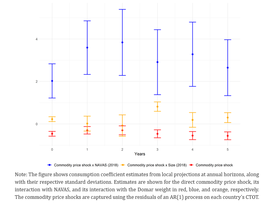
Following a positive CTOT shock, countries with higher NAVAS experience stronger positive consumption responses (Figure 3). The amplification effect of NAVAS for TOT shocks is statistically significant and robust across horizons (blue line) while the effect of sector size on the transmission of TOT shocks is modest and often insignificant (orange line).

Figure 3. Effects of CTOT shocks on consumption

Model-based Analysis: Income and Wealth Effects of TOT shocks

To better understand the economics underlying these empirical results we build a small-open-economy dynamic stochastic general equilibrium model based on Silva and others (2024). In the model, households consume a final composite good produced with labor, commodities, and imported and domestic intermediate goods. Households save in foreign assets which accumulate in line with the small open economy’s successive current account surplus/deficit. The real interest rate is given and fixed. Calibration uses the same OECD data as featured in Figure 2 – covering 66 countries and 44 sectors – and is set to match each country’s sectoral final consumption shares, IO shares, and the commodity sector’s net exports, all in 2018.

Once calibrated, the model is used to investigate the relationship between NAVAS and the co-movement between consumption and commodities terms of trade. Model simulations in Figure 4, panel 2 show results that are very similar to the raw data correlations depicted in Figure 2, panel 2: the slope is positive (EMDEs tend to have both higher NAVAS and higher correlation of cyclical consumption and terms of trade shocks), and some AEs do display higher NAVAS and stronger co-movement than EMDEs. In contrast, when model-based consumption responses are plotted against the commodity sector’s size (Figure 4, panel 1), no clear relationship emerges and the cloud of points hovers around a horizontal line at 0, suggesting that NAVAS is a better summary statistic to explain cross-country variations in consumption volatility.

Changes in a country’s terms of trade affect the economy in two main ways: by influencing people’s incomes through real wages, and by shaping the real financial gains or losses that ultimately flow to households – the country’s net foreign asset position (NFA). The way NAVAS affects these two channels, especially the NFA channel, shapes how interconnectedness influences the transmission of TOT shocks.

Figure 4. Model-based consumption responses to a TOT shock against size and against NAVAS

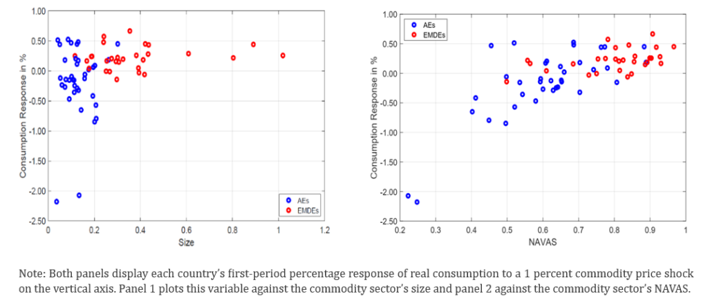
An increase in commodity prices affects the valuation of the NFA position on impact and its dynamic response. When foreign assets are denominated in commodity units, the real value of NFAs increases more in countries with higher commodity sector NAVAS (for more details, see Gomez-Gonzalez and others, 2025). The increase in the real NFA position creates a positive wealth effect in commodity-exporting economies, usually EMDEs (in red), increasing consumption on impact. In contrast, many AEs (shown in blue) experience a negative consumption response. Because they are commodity importers, the real value of their debt (in commodity terms) is increased by the shock, leading to a negative wealth effect.2

Conclusion

The macroeconomic impact of commodity price shocks on consumption depends less on the size of the commodity sector than on how connected it is with the rest of the economy. The network-adjusted value-added share (NAVAS) captures this interconnectedness and explains cross-country differences in the response of consumption to commodity price fluctuations, with an emphasis on income and wealth effects. The commodity sector’s NAVAS shapes the strength of wage responses (income effect) and the downstream propagation of commodity price shocks to the consumer price index with implications for the valuation of net foreign assets in real terms (wealth effect).

This has important implications for policymakers across both advanced and emerging markets and developing economies. And this is particularly important for central banks (Qiu and others, 2025). Because the inflation–consumption trade-off may depend critically on the degree of interconnectedness of the commodity sector, macroeconomic frameworks should be adapted to account for the structure of domestic production networks (Aoki, 2001; IMF WEO chapter 2, October 2024). Moreover, as terms-of-trade shocks revalue the stock of national wealth with consequences for consumption and inflation, external balance sheets and valuation channels should play an important role in policy models.

Finally, structural and fiscal policies can meaningfully shape macroeconomic resilience by altering network exposure. Policies that diversify input sourcing and strengthen domestic non-commodity supply-chain exposure can lower NAVAS and mitigate the impact of future commodity shocks. Conversely, industrial strategies that deepen domestic linkages to commodity sectors may increase exposure to global commodity price cycles, even when headline commodity dependence appears modest.