A choice-based approach to the measurement of inflation expectations

Abstract
Economists widely rely on measures of inflation expectations and uncertainty elicited via density forecasts. This approach, which asks respondents to assign probabilities to pre-specified ranges, has proven informative, but also faced criticism in recent periods of elevated and volatile inflation. We propose a method to elicit the full distribution of inflation expectations that is rooted in decision theory and can be implemented in standard surveys. In several empirical applications we demonstrate that the proposed method leads to well-defined expectations that fulfil both subjective and objective quality criteria. The method is neither perceived as more difficult nor does it take more time to complete compared to the current standard. In contrast to density forecasts, the method is robust to differences in the state of the economy and thus allows comparisons across time and across countries. It is portable and can be applied to elicit different macroeconomic expectations.

Choice-based measurement of macroeconomic expectations

Policy makers and researchers have been increasingly paying attention to households’ and firms’ expectations about macroeconomic variables, such as inflation, as indicators and tools of monetary policy, as well as essential input in theoretical models. Two moments of these beliefs have been shown to be essential (see for example Coibion et al., 2024): An average estimate of future realizations (known also as a point forecast) as well as uncertainty about the future forecast. A standard tool to elicit such expectations are density forecasts: a probabilistic question format in which respondents are shown several pre-defined intervals (or ‘bins’) and are then asked to attach probabilities to the intervals according to their beliefs about the future rate of inflation. This format was popularized in the Survey of Consumer Expectations (SCE) by the Federal Reserve Bank of New York and implemented by several other major central banks.

However, the recent surge in inflation has not just shown the importance of data on subjective probabilistic beliefs to gauge individual-level uncertainty but has also exposed challenges to the measurement through density forecasts. One concern is that density forecasts are very sensitive to the response scale. During periods of high and volatile inflation, response-scale framing effects may bias measurements, and responses may also end up being lumped in extreme (open) bins. Another concern regards the typical bin structure: narrower bandwidths around zero may induce survey participants to perceive that values close to zero are considered more likely by the designers of the survey, which may bias responses towards zero. These issues have no easy solution, because adjusting the size and value of bins across survey waves makes it difficult to compare survey responses over time. The same holds for comparisons across countries with different inflation regimes.

To overcome these issues, we propose to elicit individuals’ subjective probability distribution over expected inflation via a midpoint method that does not provide any external frames, avoiding the above described problems of density forecasts. The approach is fully driven by a respondent’s answers. It is based on simple binary choices and does not refer to the concept of probability. It is portable across times and countries with different inflation regimes. Moreover, if a survey elicits expectations for several variables (interest rates, unemployment rates), it is not necessary to provide several bin structures tailored to the respective variables: the method can be applied to each of the variables of interest in the same way.

Midpoint method

The midpoint method is based on Baillon (2008) and consists of a binary choice-based bisection process that partitions the space of possible outcomes into equally likely subevents, from the perspective of the respondent. The method starts by asking the respondent for a minimum and maximum level of inflation for which they think that there is “almost no chance” that actual inflation will lie outside the interval. This avoids inducing external anchors. It then proceeds to elicit two complementary events that range from the minimum to the median, and from the median to the maximum. From this twofold partition of the space of possible outcomes, a fourfold partition one can be generated by again splitting each of the two events into two equally likely subevents, from which the 25-% quartile and 75-% quartile of the respondent’s belief distribution can be inferred. If desirable, the process can be continued by further splitting up (some of the) elicited quartiles to elicit a more fine-grained distribution.

To elicit each percentile, the respondent answers a set of chained choices, indicating in each step which of two events for inflation she considers more likely. For the median, the initial comparison concerns the two events (1) ranging from the minimum to the midpoint of the interval from the minimum to the maximum perceived possible inflation rate, and (2) from the midpoint to the maximum. The initial midpoint is thus half the distance between the minimum and the maximum perceived rates. The bisection process continues with the goal to find some midpoint for which the respondent considers the two events approximately equally likely.

The calculation of the next midpoint depends on whether the respondent considered the event with lower or higher inflation rates more likely. If the event with lower rates is chosen, the next midpoint is set as half of the distance between the minimum and the previous midpoint. If the event with higher rates is chosen, the next midpoint is set as half of the distance between the previous midpoint and the maximum. Intuitively, whenever an event is considered more likely, the range of that event is reduced for the following question.

This bisection process continues until a predetermined level of precision between the two most recent midpoints is reached. The final midpoint then represents the point for which subjects consider each of the two events approximately equally likely, thus representing the median of the subjective probability distribution. The process continues to identify the 25th-percentile of the respondent’s subjective belief distribution by splitting the interval between the minimum and the elicited median in the same way with the above-described algorithm; similarly, for the 75th-percentile and any further percentiles the researcher wants to identify.

Midpoint method: Example

Table 1 gives an illustration of the bisection process, assuming a desired precision of 1.5%. A hypothetical respondent indicates that she expects the lowest possible rate of inflation to be 0% and the highest possible rate to be 20%. Based on this interval, the first midpoint is 10%. The respondent indicates option B as more likely (that is, she believes a higher rate of inflation is more likely), implying the second midpoint of  (20% + 10%)/2 = 15%. Based on the two events that follow from the second midpoint, the respondent prefers option A, which leads to the next midpoint of  (15% + 10%)/2 = 12.5%. Given that the desired level of precision is not yet reached (15% -12.5% > 1.5%), the elicitation process continues, and the respondent again prefers option A. The next midpoint equals (12.5% + 10%)/2 = 11.25%. It satisfies the precision criterion as it is less than 1.5% different from the previous midpoint. This concludes the first bisection process, and the final midpoint of  11.25% serves as the median of the inferred subjective probability distribution.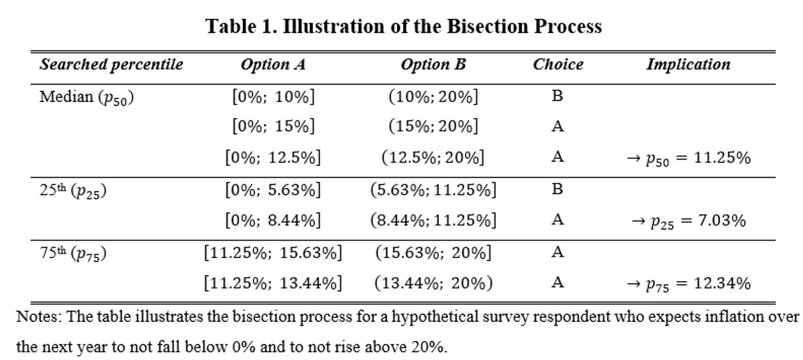

The process continues with the elicitation of the 25th-percentile. The first midpoint of (0% + 11.25%)/2 = 5.63% is calculated from the minimum and the median As the respondent prefers option B, the next midpoint is  (5.63% + 11.25%)/2 = 8.44 From the next set of options, the respondent prefers A, implying the next midpoint of (5.63% + 8.44%)/2 = 7.03%, which already satisfies the desired level of precision. It serves as the 25^th-percentile. Finally, the process concludes with the elicitation of the 75^th-percentile in the same way.

Empirical implementations of the midpoint method

To gauge the performance of the midpoint method in the field, we conducted two surveys in the U.K. in 2023 and the U.S. in 2024. In the U.K. survey, we focused on testing the feasibility of the method in comparison to the density forecast format anchored around zero (as in the SCE) and a shifted version anchored around respondents’ own point forecasts. In the U.S. survey, we additionally focused on testing the quality of the elicited distributions by including control questions based on respondents’ own responses, and a randomized controlled trial (RCT) that allocates respondents into groups with different information to generate exogenous variation in their inflation expectations. We use this variation to study the causal effects of the resulting change in expectations, as measured by the two different elicitation formats (midpoint versus density forecast), on spending.

Our results show that the midpoint method is perceived as easy and fast as the density forecast. Actual response times were similar in the U.K., and faster in the U.S. survey for the midpoint method. We find notable differences in the distribution of subjective inflation expectations depending on the elicitation method. The Midpoint method elicits inflation expectations with substantially higher implied means and higher disagreement than the SCE probabilistic question format, but similar implied means and disagreement as the shifted probabilistic format. The Midpoint method also delivers significantly lower forecast uncertainty relative to methods relying on density forecasts.

We also find that the Midpoint method leads to a higher correlation between implied mean forecasts and respondents’ point forecast relative to the probabilistic question format of the SCE. Moreover, when inflation expectations are elicited through the midpoint method, only 2% to 4% of the total probability mass (depending on the survey) is allocated to deflation scenarios. In contrast, when inflation expectations are elicited through a probabilistic question format, 10% to 17% of the total probability mass is allocated to deflation scenarios.

Since it is difficult to judge whether these differences indicate a better performance of the Bins or the Midpoint method, we added two quality measures in the U.S. survey. First, we confront respondents with statistics obtained from their own answers (without telling them where the statistics come from). We calculate in real-time the implied median and the implied deflation probability from respondents’ answers and then let them judge whether they broadly agree with the number, or whether they believe the number should higher or lower. For both statistics, we find that that a larger share of respondents in the Midpoint treatment agrees with statements derived from their own previous answers. In contrast, the Bins SCE method seems to elicit too large probabilities of deflation, which then biases the implied median downward and leads to overall lower agreement by the respondents on both questions. For the midpoint method we find that it seems to elicit too low probabilities of deflation, although the disagreement of respondents with their own expectations is less pronounced than for the SCE density forecast.

Second, we assess the causal effects of how well elicited inflation expectations map to respondents’ consumption choices by making use of the RCT design. We measure durable consumption intentions using three items that have been used by prior studies and in which a positive relation to subjective inflation expectations is expected. When post-treatment inflation expectations are elicited using the Midpoint method, we find a positive and statistically significant effect on all three durable consumption categories. In contrast, when inflation expectations are elicited using the SCE density forecasts, we find effects that are often insignificant and of different sign across categories.

A final test benchmarks the methods against an objective underlying distribution. The main concern is that the true beliefs of respondents are unobserved, and that it is difficult to draw conclusions on how well they have been measured. To circumvent this, we designed an experiment in which participants can repeatedly sample (positive and negative) numbers from one of two underlying distributions and afterwards report their beliefs regarding the sample using either the SCE bins or the Midpoint method. We find that the Midpoint method elicits beliefs that better approximate both the mean and the standard deviation of the underlying distribution. In terms of the probability of a negative number (akin to deflation probability), we find that the Midpoint method underestimates this probability, while the Bins SCE method strongly overestimates it, driven by the inappropriate use of “negative” bins. This finding is consistent with our survey evidence on the use of deflation bins. The severity of the biases in terms of deflation probability in surveys thus depends on the underlying distribution. If a country faces little to no deflation, the bias in the Midpoint method will be rather small while the bias of the bin method can be sizable, as documented in our two surveys.

Practical considerations

We close by discussing several practical issues that may become relevant in applications of the proposed midpoint method.

Wide range between minimum and maximum. Respondents may initially indicate a very large interval of possible inflation rates. This does not harm the precise elicitation of the different percentiles, but the process may require more steps to reach the required precision. However, for the calculation of implied means and uncertainty from the elicited distribution, the assumption of a uniform distribution within percentiles is often made. This assumption may not be a good approximation in this case. Consider the example in Table 1. The respondent may have indicated a maximum of 20% because she believed there is a very small probability that inflation may run very high over the next year; overall though she may consider the probability that inflation will be above, say, 15% close to zero. With her fourth quartile ranging from 12.34% to 20%, we would possibly make a substantial error in the calculation of the implied mean assuming uniform distribution within that bin, given that most probability mass is actually close to its lower bound of 12.34%. The problem is that the quartile is still too wide, providing too little information.

This problem can be resolved by adding additional layers of subdivision as long as an elicited percentile is still considered too wide. In the example, splitting the forth quartile by eliciting the 87.5th percentile would reduce the problem by immediately allocating half of its probability mass to values close to 12.34%.

Random choices in later elicitation steps. Initial choices may be rather clear for respondents. However, as we approach indifference in the sequence of choices, it may become more difficult for the respondent to say which interval she considers more likely, and she may revert to answering randomly. This feature is inherent to the method and the idea of indifference. However, if researchers find it desirable that respondents can indicate that they find it difficult to decide between the two intervals, an endogenous stopping opportunity may be added through an “I consider both intervals equally likely” option.

Midpoints exactly equal to elicited percentile. A related issue concerns the case where a midpoint is exactly equal (or very close) to the elicited percentile. In this case, again, the respondent should indicate indifference directly. If we do not want to offer this possibility, a forced choice approach will initially move the midpoint away from the true value. However, in each subsequent step, the midpoints will then converge back in the direction of the true value of the elicited percentile. The induced error depends on the level of precision chosen by the researcher.

Error propagation along the elicitation chain. Because of the chained structure of the method, any errors early in the process will propagate through the whole sequence, affecting values elicited later. For example, if the median is assessed with error, the 25%- and 75%-quartiles will also be assessed with error. Error propagation cannot be prevented in the method, but it is unclear how severe the problem may be compared to errors in the elicitation using bin-based density forecasts. Errors can be mitigated by choosing a higher precision, allowing the process to converge back to the true value after an error. A higher precision in earlier stages of the process (notably the elicitation of the median) may be warranted to mitigate the problem in later stages.