Real-time fiscal monitoring with Bayesian VARs

Key messages

• Fiscal monitoring entails forecasting key fiscal variables such as the government deficit-to-GDP ratio, providing a narrative for their dynamics and constructing scenarios.
• This brief describes an approach based on a parsimonious Bayesian mixed-frequency VAR that combines monthly cash-flow data from the Treasury with macroeconomic and financial indicators.
• Applied to Italy (2010–2023), the model produces monthly nowcasts that match or outperform European Commission point forecasts — using only 11 variables and no expert judgment.
• In scenario analysis, a monetary tightening raises the deficit substantially more than a same-sized “typical” recession, because falling interest rates in the latter dampen expenditure growth.

Why fiscal monitoring matters more than ever

Global public debt is elevated and set to rise over the medium term (Dabla-Norris et al., 2025). In Europe, new spending pressures — defence, the green transition, and support for industries facing geopolitical headwinds — are adding to already high debt stocks, while rising yields tighten financing conditions. In this environment, detecting early signs of fiscal stress and translating them into actionable policy narratives is more important than ever.

Yet the institutional infrastructure for tracking fiscal developments in real time has clear gaps. Official forecasts of the government deficit-to-GDP ratio are published only twice a year (in spring and autumn by the European Commission), leaving policymakers without timely signals for months at a time. Underlying fiscal data are also released with long lags: quarterly government revenues and expenditures typically become available only four months after the reference quarter, and are subject to sizeable revisions (Cimadomo, 2016).

In this brief we summarise a new, data-driven framework for fiscal monitoring that addresses these gaps. The approach builds on the mixed-frequency Bayesian vector autoregression (VAR) introduced in Cimadomo et al. (2022), extended to the fiscal domain, and is illustrated through an empirical application to Italy — a natural test case given its high debt-to-GDP ratio and the fact that its monetary policy is set at euro area level.

How the model works

Nowcasting the deficit ratio effectively requires mapping out the dynamics of three quarterly variables — government revenues, government expenditures, and nominal GDP — which are released with different and considerable delays. We develop a mixed-frequency model to handle this complexity.

Combining slow and fast data. Two types of fiscal data exist but are rarely combined in a coherent model. Accrual data (quarterly revenues and expenditures, consistent with national accounts) measure what matters for the deficit ratio, but arrive late. Cash data (monthly inflows and outflows recorded in the Treasury account) are available within two months of the reference period, but are noisier and cover only the central government. The key insight is that the two are correlated: cash flows carry timely, if imperfect, signals about the accrual aggregates that will be published later. A model that learns this relationship can use cash releases to continuously update its deficit outlook.

The Bayesian mixed-frequency VAR. The model (Cimadomo et al., 2022) casts all variables — quarterly and monthly — into a unified monthly VAR framework by treating low-frequency observations as higher-frequency series with missing values at the intra-quarter level. The system includes 11 variables: quarterly real GDP, the GDP deflator, and general government revenues and expenditures (accrual); and monthly cash revenues and expenditures, consumer prices (HICP), the 10-year Italian bond yield, industrial production, economic sentiment, and an industrial turnover index. We estimate the model with Bayesian techniques and handle the mixed-frequency structure and the “ragged edge” associated with real-time data releases through Kalman filtering and smoothing.

We apply our model to 208 real-time monthly data vintages for Italy (January 2007 to April 2024), mimicking the exact information set a fiscal analyst would have on the 15th of each month. This allows us to evaluate model performance under the same information constraints that practitioners actually face.

Nowcasting the Italian deficit: results

Figure 1 summarises the main nowcasting results over 2010–2023. Three features stand out.

First, the model tracks the deficit ratio closely across a wide range of conditions. From 2010 to 2019 — a period covering the sovereign debt crisis, fiscal consolidations, and a tentative recovery — the median BVAR nowcast stays close to the outturn, with uncertainty bands that narrow systematically as the year progresses and more data arrive.

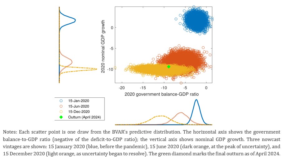
Second, the model responds quickly to large shocks. When Covid-19 struck in 2020, pushing the deficit from around 1.5% of GDP in January to nearly 9% by year-end, the BVAR began revising upward already in May 2020 — as soon as cash and high-frequency macro data started reflecting the collapse in activity — and by June was already assigning substantial probability to outcomes that had never been observed in the sample. Figure 2 illustrates this vividly: the joint distribution of GDP growth and the government balance shifts dramatically between January and June 2020 and then tightens again by December as uncertainty resolves.

Third, despite using only 11 variables and no expert judgment, the BVAR matches or outperforms the European Commission’s forecasts in most months of the nowcasting horizon. This is a striking result given that the Commission’s projections draw on nearly 200 variables, multiple models, and the judgment of seasoned fiscal and macro economists who are likely informed by budget plans not yet reflected in public data. The one period of sustained underperformance for both the BVAR and the Commission — 2022 and 2023 — reflects the massive and unanticipated ex-post revisions triggered by the Italian “Superbonus 110%” building incentive scheme, whose full fiscal cost (eventually estimated at around €160bn, or 8% of GDP) was recognised in public accounts only with a substantial lag.
A further practical advantage is that the model produces a monthly update of the deficit outlook, filling the information gaps of up to six months left between the semi-annual rounds of official forecasting — exactly the periods when early warnings matter most.

Figure 1. Nowcast of the Italian deficit-to-GDP ratio: BVAR vs. European Commission and final outturn, 2010–2023

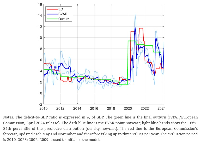
Figure 2. Joint nowcast of GDP growth and government balance ratio during the Covid-19 crisis (2020)

Scenario analysis: monetary vs. typical recessions

Beyond tracking the fiscal outlook, the model supports counterfactual scenario analysis. We compare two recession scenarios calibrated to produce the same peak-to-trough decline in Italian GDP:

• Monetary recession: GDP falls because of an exogenous monetary policy tightening, identified using the market-surprise approach of Jarociński and Karadi (2020), which separates pure interest-rate shocks from central bank information signals.
• Typical recession: GDP falls by the same amount but is driven by the business-cycle shocks that normally account for most of the variation in Italian output.

Figure 3. Response of the deficit-to-GDP ratio to a monetary recession (left) and a typical recession of equal GDP magnitude (right)

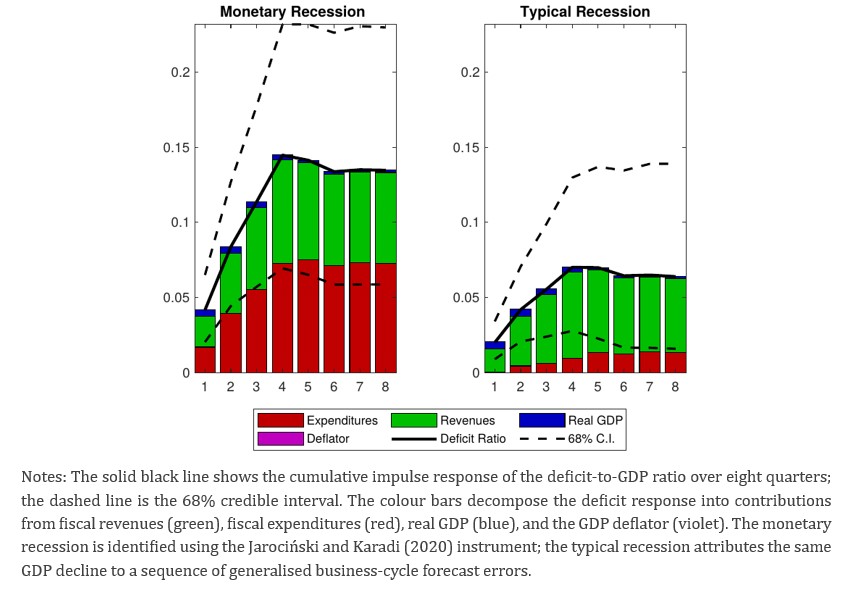
In the monetary recession (left panel, Figure 3), the deficit-to-GDP ratio rises by around 13–15 basis points and remains persistently elevated. The increase is driven by two forces pulling in the same direction: revenues fall as the tax base contracts, while expenditures rise — partly through automatic stabilisers (unemployment benefits, etc.) and partly because higher interest rates directly raise debt-servicing costs.

In the typical recession (right panel), the deficit also rises, but the response is substantially more muted — roughly half the size. The key difference is that in a typical recession, monetary policy responds endogenously by lowering interest rates to stabilise the economy. As a result, while fiscal revenues fall by a similar amount, fiscal expenditures increase much less because the interest bill actually falls. Automatic stabilisers still operate, but their effect on the deficit is partly offset by the relief on debt service.

This comparison carries a direct policy message for the current conjuncture: a monetary tightening cycle — such as the one the ECB pursued in 2022–2024 — generates a fiscal cost substantially larger than what a model calibrated only to historical recessions would predict. Countries with high debt ratios, such as Italy, are especially exposed, since their interest expenditure is more sensitive to rate movements.

Policy implications and broader applications

The framework fills a genuine gap in the toolkit available to fiscal analysts and policymakers. It provides:

1. Timely monthly updates of the deficit outlook, between the semi-annual rounds of official forecasting institutions.

2. Density forecasts that quantify the risks surrounding the central projection — not just a point estimate.

3. An economic narrative through “news” decompositions that attribute revisions in the deficit nowcast to specific data releases, allowing analysts to identify whether a deterioration is driven by the revenue side, the expenditure side, or macroeconomic developments.

4. Scenario analysis that captures how different types of shocks transmit to the fiscal balance through both revenue and expenditure channels, including the endogenous response of monetary policy.

The approach is not Italy-specific. It can readily be applied to any country for which monthly cash data and a standard set of macro indicators are available — including other high-debt euro area members, the United States, the United Kingdom, or Japan, all of which face growing fiscal pressures. The model’s performance during the Covid-19 crisis — where it quickly identified an unprecedented deterioration in the fiscal outlook — suggests it is particularly valuable precisely when timely and reliable fiscal signals are most needed.