menu
close

Author(s):

Claudio Borio | Bank for International Settlements (BIS)

Keywords:

Natural interest rate , central banking , monetary policy

JEL Codes:

E40 , E43 , E52 , E58

The concept of the natural rate of interest, or r*, has risen to prominence in monetary policy following the Great Financial Crisis. No doubt a key reason for the concept’s newfound prominence has been the further decline of real and nominal interest rates to new lows, which has further constrained monetary policy’s room for manoeuvre. This lecture explores the extent to which the concept can be a useful guide to policy. It concludes that, depending on how it is employed, the concept has the potential of leading policy astray and of complicating the task of regaining the needed policy headroom. If so, within a credible policy regime, there is a premium on flexibility in the pursuit of tightly defined inflation targets – on tolerance for transitory, but possibly persistent, shortfalls of inflation from target.

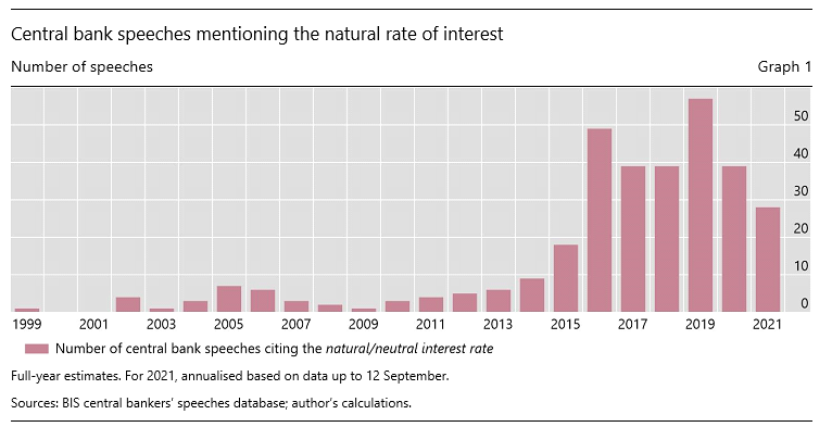
The concept of the natural rate of interest, or r-star (r*), has risen to prominence in monetary policy following the Great Financial Crisis (GFC). The frequency of references in central bank speeches attests to that (Graph 1).3


 width=

Prior to the GFC, the concept was much better known in academia than in policy circles. The notion had been “rediscovered” with the development of New Keynesian models (eg Woodford (2003)) after having largely fallen out of fashion in the post-war era, overshadowed by Keynesian economics and monetarism’s primary focus on monetary aggregates.

No doubt a key reason for the concept’s newfound prominence has been the historically unusual behaviour of interest rates. Nominal interest rates have been extraordinarily low – the lowest since historical records began. And real interest rates have been negative for even longer than during the Great Inflation era – and probably since records began, too. Monetary policy has been significantly constrained as a result.

When considering the concept’s increased prominence in policymaking, it is worth making a distinction. The increase does not so much relate to the concept’s use in the setting of the monetary policy stance on a regular basis, but to its influence on communication, strategies and, more recently, the review of monetary policy frameworks (Powell (2020), ECB (2021)). Indeed, a key motivation for the reviews has been the need to increase the room for policy manoeuvre in a world in which r* has fallen substantially owing to structural factors.

Because of its renewed prominence, it is worth examining the concept in depth as a guide to policy: to put it more bluntly, is it safe or hazardous to navigate by r*?

I would like to explore this question very much from my personal perspective. This will allow me to stretch the boundaries further, be more provocative and trigger a richer discussion.

Let me stress three takeaways from my presentation.

First, r* is very imprecisely estimated and contains little information beyond that provided by other variables, such as potential output or the natural rate of unemployment. As a result, r* is not really needed when setting the policy stance ex ante, although it can play and does play a role when interpreting the stance ex post. I think there is broad agreement on this point.

Second, and more controversially, because of its defining features and depending on how it is employed, r* has the potential of leading policy astray. In particular, the view that r* is independent of monetary policy and not much affected by purely financial factors could complicate the task of regaining policy headroom over time (Borio (2021)).

Finally, should these propositions be valid, there would be a case for greater flexibility in the pursuit of inflation objectives, within credible policy regimes, in order to rebuild the needed monetary policy headroom. By flexibility, I mean tolerance for transitory, but possibly persistent, deviations of inflation from narrowly defined targets. In other words, central banks would have greater degrees of freedom than the r* concept would suggest.

The rest of the presentation is organised as follows. The first section elaborates on the concept of r*. The second assesses its possible role as a policy guide. The final one draws some policy implications.4

The concept

The concept of the natural rate of interest goes back a long way in the history of economic thought. While it is most closely associated with Wicksell (1898), the seeds of the idea can already be found in John Stuart Mill.

The natural interest rate is generally defined as the short-term real interest rate that, in the absence of shocks – in steady state – equates saving and investment, clearing the goods market at the level of output that corresponds to potential. At that point, inflation is seen as stable. In addition, in virtually all representations, r* is independent of monetary policy and driven exclusively by structural factors.

Three implications follow. The natural rate of interest is a purely notional and unobservable variable; it is intimately linked to a specific view of the inflation process, in which economic slack plays a key role; and it is beyond the influence of monetary policy.

Importantly, the “existence” of such a rate does not imply that saving and investment directly determine any market interest rate. In fact, I would argue, quite plausibly they do not.

There are two theories of the determination of market interest rates in Economics 101. The first is the loanable funds theory. In this case, the supply and demand for funds determines interest rates5 – a view that, over time, has morphed into the statement that the real interest rate is determined by saving and investment (eg Mankiw (2013)). This is a flow view of market interest rates. The second is the liquidity preference or portfolio view. In this case, the interest rate equates the supply of, and demand for, different assets, notably “money”. This is a stock view. It harks back to Keynes (1936) and Hicks (1967) and is embodied in the famous IS-LM stylised representation of the economy.

In fact, we know that the actual determination of market interest rates does not quite correspond to either approach, although it is closer to the second. We know that the central bank sets the short-term (overnight) nominal rate in the market for bank reserves, over which it has a monopoly. It does so through a mixture of signals and liquidity management operations – this is indeed a stock equilibrium (eg Borio (1997), Bindseil (2004)). At longer maturities, the influence of the central bank, while still potentially pervasive, is more limited, as the unconstrained portfolio decisions of market participants play a much bigger role. Critically, in this case the central bank sets the tone by influencing expectations of the future path of the short-term rate. Beyond that, supply and demand factors, including central bank outright purchases, determine term, liquidity and any credit risk premia. Because the prices of goods and services are largely predetermined, nominal interest rates also determine the ex post real rates and, together with sluggish inflation expectations, ex ante real rates.

Importantly, this is true at any given point in time; logically, it must also be true at all points in time. Put differently, small risk premia aside, it is the central bank that always determines the short-term market real interest rate. To be clear, I do not mean that, today, the central bank can set the whole structure of real interest rates: its influence on nominal rates wanes along the curve (unless it intervenes directly) and that on market participants’ inflation expectations is more limited, in part depending on its credibility. What I do mean is that, when tomorrow comes, the central bank can set the short-term rate at that point, and the same is true at all future dates.

It then follows that r*, and hence saving and investment, play no direct role in the determination of the short-term market rate. At any given point in time, saving and investment adjust to the policy rate. They influence the market real interest rate only through the central bank’s rate-setting decisions in response to economic developments – the reaction function.

What, then, can people really mean when they say that “the central bank does not set the (short-term) real interest rate in the long run”? The statement cannot be literally true unless, as is analytically often done, it is assumed that prices are fully flexible – a kind of jump variable – at that point.6 It can only logically mean that the central bank is forced to set a market interest rate in line with a specific rate, r*, that is beyond its control.

But why? Presumably because, if the central bank does not set a market interest rate consistent with r*, something will give way, ie the economy will “veer off track” and induce or compel the central bank to adjust (Borio (2017)). Given the definition of r*, the unwelcome development that takes the economy off course is output moving away from potential, which has a proportional relationship with changes in the inflation rate (all else equal). In fact, a rather extreme version of this property is embodied in New Keynesian models: any small deviations of expectations from r* at some future horizon prompt an explosive inflation or disinflation.
In other words, r* is like an invisible hand that guides policy to the right destination. Note, though, that there is a key difference between potential output and inflation. Potential output, just like r*, is unobservable, while inflation can be observed directly. As we shall see shortly, this is far from inconsequential for practical policymaking.

Guide to policy

What are the desirable properties of any policy guide and hence also of r*? The guide should be, first, measurable with sufficient precision and, second, consistent with good economic outcomes.

These two properties play different roles. The first is essential for r* to be useful as a guide when setting the policy stance within a given strategy. The second, which matters regardless of the first, is what determines whether r* is useful in shaping the strategy itself and the framework under which that strategy is chosen. It is this aspect that embodies fundamental views about how the economy works, over which, naturally, there can be justifiable disagreement.

Consider each aspect in turn.


Measurement

Since r* is unobservable, it must be estimated, and any estimation must be based on some “model”.

There are essentially three approaches.7 The first and simplest is to use purely statistical properties of the data. This approach ranges from different types of weighted averages, which smooth out interest rates over long periods (univariate filters), to multivariate unobserved component models. The idea is that this can roughly approximate the steady state. The second is to back out r* based on additional economic information, of various degrees of richness. For example, it is common to filter out r* from a system of structural relationships assumed to hold in the data. Such systems invariably include an IS-curve, linking output to the real interest rate, and, critically, a Phillips curve, linking inflation to measures of economic slack, notably an output gap. The third is to use more sophisticated market proxies, which capture the expectations of market participants, eg a real forward rate out in the yield curve. The idea here is that market participants, on average, are right and that such a forward rate is beyond the direct control of the central bank.

The dominant approach is the second. In this case, regardless of the specifics, a key piece of information is the behaviour of inflation.8 All else equal, if inflation rises, output must be above potential, so that the real interest rate must be below r*. The opposite is true when inflation falls. As a result, as is well known, it is quite common to adjust measures of potential output based on the behaviour of inflation. In particular, if output looks way above trend, but inflation fails to rise, potential output is adjusted upwards. The same is true for other unobservable variables, notably the natural unemployment rate, which can enter the model through additional relationships, eg Okun’s law.

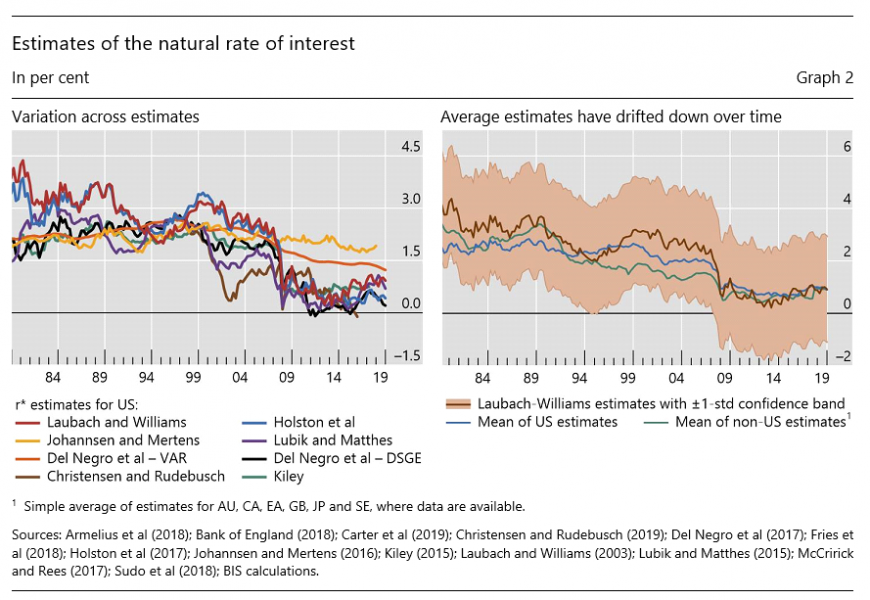
The combination of different approaches and estimation techniques means that it is very hard to pin down r* (Graph 2). The estimates differ substantially across methodologies (left-hand panel). And, for any given methodology, they are subject to substantial estimation uncertainty. To give a sense of the imprecision, the standard errors around the well known Laubach-Williams natural interest rate estimates span 2.5 percentage points (right-hand panel). In other words, at most points in time, it is hard to say with any certainty whether interest rates are above, below or at r*.

 width=

The estimates are bound to differ widely across approaches because of the variety of inputs used. In some cases, the difference may in fact be welcome. For instance, it would be unfortunate if estimates that brought essential economic information to bear in order to adjust univariate statistical filters yielded very similar results. This would mean that those economic relationships carry little information. In other cases, differences across approaches may be more troubling. Arguably, one such example is comparing market participants’ estimates derived from the yield curve with more model-based ones. The policymaker would need to decide relying on the relationships that they find most useful. Hence the importance of the link between economic slack and inflation – the slope of the Phillips curve.

For a given approach – to be more precise, fundamentally similar “models” within that approach – the imprecision reflects the reliability of the economic relationships on which the inferences are based.9 Those economic relationships may themselves be imprecisely estimated, unstable or contain little information.

It is here that the Phillips curve plays a key role. A link between economic slack and inflation is bound to exist. The problem is that the relationship has been quite elusive. And when estimates are statistically significant, they indicate that the sensitivity of inflation to economic slack is very low – the Phillips curve is “very flat”.10 This amplifies the impact of any estimation errors on r* estimates: a given inflation outcome is consistent with a range of values for r*. To complicate matters further, the results are sensitive to the treatment of trends in the observable variables and “shock” processes, which adds another degree of freedom (Lewis and Vazquez-Grande (2019)).11

Despite disagreement on the level of the natural rate, most methods reach the same conclusion: r* has fallen since the early 1980s (Graph 2, left-hand panel). This is not that surprising. Real interest rates have indeed come down substantially, and r* estimates are generally constrained not to deviate too much from those rates – nor would a very different answer be regarded as credible. Moreover, inflation has been pretty stable below target for a long time despite central bank efforts to push it up: the estimation methods interpret this as indicating that the stance is not sufficiently expansionary, ie that the policy rate is not sufficiently below the natural rate. Indeed, the estimates predicated on the Phillips curve tend to yield the steepest decline in r*. By contrast, those for which the decline is less obvious derive r* from market expectations and allow the term premium to move a lot along significant trends, eg Brand et al (2020) and Davis et al (2021).

This evidence suggests that r* is ill suited as a guide for setting the policy stance in real time. Not only are the estimates very imprecise, but r* contains little information over and above that contained in other unobservable variables, such as indicators of economic slack – typically the output gap or the natural level of unemployment, from which r* is typically derived. To be sure, those estimates are themselves subject to considerable uncertainty: just as r*, they raise questions about the desirability of relying heavily on them in policymaking. Regardless, though, they are much more directly linked to inflation forecasts. As a result, when setting policy, it is quite possible, and common, to forecast inflation and adjust interest rates without explicit reference to r*. In that case, r* would at most be indirectly used as part of robustness checks, such as when gauging the policy stance with respect to Taylor rule benchmarks (the intercept). Consistently with this general approach, r* was hardly mentioned pre-GFC.

By contrast, post-GFC r* has played a more prominent role in communication. Several central banks have relied on the notion to convey various ideas: when rates have been extraordinarily low, to indicate how far “normalisation” may have to go (eg Williams (2018), Debelle (2017)); ex post, to assess whether monetary policy has been accommodative or restrictive; and, more generally, to underline the message that structural factors beyond the central bank’s control have pushed interest rates to such low levels over the long term. The concept is clearly much better suited for such uses.


Good economic outcomes

When assessing whether r* as a concept facilitates good economic outcomes, the view that r* is independent of policy is key – a view embedded in the broader notion of the neutrality of money.

This view has the big merit of underlining, rightly, that monetary policy is not all-powerful. Certain deep-seated long-term features of the economy are beyond its influence, let alone control. For instance, ultimately if one wishes meaningfully to increase long-term growth, other policies need to do the heavy lifting, notably structural reforms and growth-friendly fiscal policy (eg BIS (2021)).

At the same time, and more controversially, taken literally, this view may take the real/nominal dichotomy too far. In particular, it may tend to overestimate monetary policy’s influence on inflation and underestimate its influence on certain features of the real economy over medium- and longer-term horizons, notably through its impact on financial factors.

Either way, the result would be similar. Depending on how the belief influences policy, it could risk reducing the room for policy manoeuvre over time. To understand why this is possible, let me consider, in turn, the inflation process and the role of financial factors in driving the economy.

The belief that r* is independent of monetary policy, if entertained, can greatly constrain the central bank when seeking to gain policy headroom and when nominal interest rates are low. Taken literally, it implies that the only way of gaining headroom on a sustainable basis is to raise inflation so that nominal interest rates can increase alongside it. This means that the central bank must cut rates (ease monetary policy) today in order to raise inflation tomorrow. Thus, paradoxically perhaps, gaining policy headroom tomorrow requires losing it today.

The problem is that, if inflation is not sufficiently responsive to monetary policy, there is a risk that policy space could diminish over time. This would occur if the hoped-for increase in inflation failed to materialise to the necessary extent. The post-GFC experience could be read in this light.

The post-GFC experience is part of a well known broader picture. It is not just that the Phillips curve has become very flat and hard to estimate. There is also growing evidence that the inflation expectations that really matter for price setting – those of workers and firms – may have substantial backward-looking elements (eg Cecchetti et al (2017)) or not be very responsive to central bank announcements, at least when inflation is low (Coibion et al (2018), Candia et al (2020)). That evidence suggests that facts matter more than words when forming views about future inflation.12

Interestingly, to my mind, the most plausible explanations for the limited sensitivity of inflation to monetary policy point to structural forces – the type of factors normally associated with r*. Especially prominent here are globalisation and technology, which have arguably reduced the pricing power of both labour and firms, muting second-round effects, and have put persistent downward pressure on inflation, especially in advanced economies.13 Such powerful headwinds can limit monetary policy’s ability to raise inflation relying exclusively on its own resources.14

So much for inflation by itself; what about the role of financial factors? Here, the interaction between the financial cycle, monetary policy and inflation takes centre stage.

In this case, the mechanism for the loss of policy headroom involves an asymmetric monetary policy reaction function: policy tightens little during business expansions but eases, possibly strongly and persistently, during contractions. With inflation low and stable during expansions, the central bank has little incentive to tighten and can afford to remain accommodative for longer to boost output and employment. Rephrasing this in terms of r*: inflation turning out to be surprisingly stable would tend to encourage upward revisions in potential output estimates and hence downward revisions in r* estimates, suggesting that monetary policy is tighter than it would otherwise appear to be and discouraging any tightening. Such a strategy would offer little counterweight to financial expansions and the possible build-up of financial imbalances, which can contribute to recessions further down the road. Hence a tough intertemporal trade-off: boosting output in the near term may run the risk of a possibly larger downturn in the longer term.

It is easy to see how this asymmetric policy response can contribute to a downward trend in nominal rates and, given broadly stable inflation, also real rates over time (eg Borio (2017)). Rungcharoenkitkul et al (2019) model such a phenomenon by combining endogenous business and financial cycles with inertia in the central bank reaction function.

Over time, this asymmetric policy response could contribute to the risk of a debt trap (Borio and Disyatat (2014)).15 If, in the process, private and public debt in relation to GDP continue to rise, over time the economy can become less able to withstand higher interest rates. This risk would be more material if the expansionary impact of interest rates on real economic activity diminishes as they become lower and stay there for longer – calling for more energetic easing when economic conditions are weak – or if debt service ratios are important determinants of expenditures – increasing the sensitivity of demand to higher rates. There is some evidence consistent with these hypotheses.16

One could see the signs of such a mechanism at work in the experience since the mid-1980s. It was then that the business cycle changed, with recessions evolving from inflation-induced to financial cycle-induced (Borio et al (2019), BIS (2021)). And such recessions tend to be deeper and longer. Ostensibly, it takes time to deal with the debt overhang and the need to reallocate resources (eg from a bloated construction sector; Borio et al (2016)). Put differently, in this new environment changes in inflation lose their significance as indicators of “disequilibrium” in the goods market at the same time as financial imbalances gain it.17

All this has at least three implications for the notion of r*. First, thinking of r* as a reliable policy guide can be hazardous since it has the potential to lead policy astray. Second, thinking of r* as independent of monetary policy may not be that helpful. What monetary policy takes as exogenous at any given point in time can be the result of past policy decisions. In this sense, there is monetary policy hysteresis (Rungcharoenkitkul et al (2019)).18,19 Finally, in a world in which financial cycles prevail, to the extent that the concept of r* is used, it would not seem reasonable to define it without reference to the financial cycle.20 In fact, taking the logic one step further, it is not entirely obvious what the interpretation of r* is when there is a different financial and business cycle in steady state associated with a specific path for the short-term real interest rate.21 

More generally, there is indeed some empirical evidence that monetary policy can have a long-term influence on real interest rates, including on standard estimates of r*. Empirical approaches that “let the data speak” over long historical spans cast some doubt on the relevance of standard saving/investment drivers. And when they examine the question of the possible role of monetary policy regimes, they find indications that they may indeed matter.

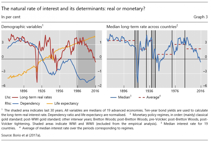
The study by Borio et al (2017a) is a case in point.22 Going back to the 1870s for 19 countries, we examine the relationship between real interest rates (a variety of measures of long and short rates as well as r* estimates), on the one hand, and the “usual suspects” (eg growth, productivity, demographics, income distribution, the relative price of capital and the marginal product of capital), on the other. We use a barrage of statistical tests.

 width=

As Graph 3 illustrates, we come up with two findings. First, while the usual suspects appear to work reasonably well over the often-cited, more recent sample that starts in the early 1980s – ie following the Volcker shock – or later, the relationships break down when going back in history (left-hand panel, which picks one of the most cited variables: demographics). Second, there are generally economically and statistically significant differences in the level of real interest rates (and possibly trends) across monetary policy regimes (right-hand panel). This is so even when one controls for the usual suspects.

How should one interpret the evidence? Surely not as ruling out a role of real interest rates in equilibrating output at potential: saving and investment drivers must matter and, to varying degrees, respond to real interest rates. Rather, the evidence suggests that many factors, well beyond “real ones”, have an important influence on that link and cloud the empirical relationships. Purely financial factors are a plausible candidate.23 This, in turn, opens the door – as it were – for a role of monetary policy regimes. In addition, the findings suggest that the widespread evidence based on calibrated models may rely too heavily on economic priors – notably by drawing on models which assume that saving and investment are driven exclusively by real factors (Borio et al (2017a)).24

Policy implications

If one took the previous analysis as given, what could be the implications for the broad direction of policy? Let me draw some personal inferences.

In my view, one could plausibly draw three such inferences. It could be desirable to: (i) have considerable flexibility when pursuing narrowly defined inflation targets; (ii) take advantage of that flexibility to re-establish policy headroom; and (iii) consider searching for complementary monetary policy guides. Let’s consider each point in turn.

By “flexibility” I mean tolerance for even persistent shortfalls of inflation from point targets unless they become uncomfortably large, endangering credibility. A sufficiently long policy horizon is essential here.

Such flexibility would help address the risk of losing, rather than gaining, precious room for policy manoeuvre – needed to address both the inevitable future recessions and unexpected costly events. The flexibility could be used to remove accommodation and regain policy headroom with a steady hand as the strength of the economy allowed as long as inflation remained within a comfortable range. One could call this strategy “opportunistic removal of accommodation” or “opportunistic tightening”25 – in effect, testing the waters.26 Critically, over time this flexibility would also help manage the intertemporal trade-offs associated with financial factors generally and the financial cycle in particular.

Flexibility would require keeping in perspective concerns that inflation would drift down in an uncontrolled manner and cause major damage to the economy once it fell persistently into negative territory – deflation. These concerns explain the worries about an unmooring of inflation expectations and a loss of credibility.

Such concerns would be assuaged if two conditions held. First, if within an established regime of low and stable inflation, self-equilibrating tendencies increased the likelihood that inflation remains range-bound. Second, if the costs of even persistent but contained negative inflation rates were not as high as typically believed.27 Some empirical evidence suggests that these conditions may hold. Take each in turn.

 width=

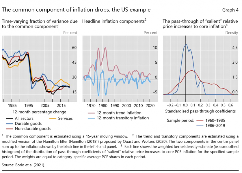
Borio et al (2021) have recently explored the behaviour of inflation at persistently low rates by looking “under the hood”, ie considering 131 sectoral prices, based on US data. The analysis points to three stylised facts: (i) the common component of inflation falls substantially relative to the sector-specific component, which becomes dominant (Graph 4, left-hand panel); (ii) the pass-through of outsize price changes to core inflation appears to be significantly lower (right-hand panel); and (iii) as already documented and consistent with those stylised facts, the transitory component of inflation grows relative to the trend component, ie persistence declines (centre panel). In other words, measured inflation appears to be largely driven by idiosyncratic price changes that have little persistent impact on its level. Hence the greater tendency to remain range-bound.28

One possible reason, which I find appealing, is the behaviour of inflation expectations. Agents may simply pay less attention to inflation when it is very low because it matters less for their decisions (“rational inattention”; Sims (2010)) – Greenspan’s (1994) very apt definition of price stability. As noted, there is evidence consistent with this view.

What about the costs of deflation? A close examination of the empirical record29 indicates little evidence of destabilising spirals – the Great Depression is an exception.30 And it also casts doubt on the existence of a systematic link between deflation and output weakness (eg Borio et al (2015) and references therein). Indeed, consistently with this perspective, some central banks have de-emphasised concerns with deflation by de facto playing down the relevance of the numerical inflation target even as inflation has been very low or persistently negative (eg the Swiss National Bank and the Bank of Thailand).

This evidence is less surprising than it may appear at first sight. After all, the impact of falling prices on activity is ambiguous a priori. Put simply, falling prices would tend to go hand in hand with increases, rather than reductions, in output when they reflect primarily improvements on the supply side of the economy (eg globalisation, technological advances, a larger labour force) rather than contractions in demand. Relatedly, any productivity growth would limit the need for hard-to-implement nominal wage cuts.31

It is, of course, one thing to point to the desirability of greater flexibility and quite another to implement it. The difficulties involved should not be underestimated. The analysis here simply indicates a direction of travel.

First, the starting point complicates matters. The exceptionally long phase of exceptionally low interest rates, underpinned by large asset purchases, has arguably made our economies less tolerant of interest rate increases. Financial markets have become more dependent on the continuation of exceptional accommodation. And debt levels – public32 and private – have risen substantially.

Second, shifting strategies is never easy. At a minimum, it would call for careful communication regarding its justification and pace in order to prepare the ground. And, depending on institutional arrangements, it may even require changes in specific mandates and agreements with the government.

Finally, what range is “comfortable” would require careful thought and is bound to be country- and circumstances-specific.

One consideration to bear in mind is that a more flexible strategy also has implications for credibility. The more precise and demanding the objective, the higher the risk of losing credibility. The other side of the coin is that greater flexibility may also make it harder to enforce accountability. In addition to helping the central bank make the right choices, complementary policy guides can play a useful role in this context.

What complementary policy guides would be consistent with the perspective outlined in this presentation? This question is worth exploring but requires further thought, both with respect to the identification of the guideposts and, even more complicated, their phasing in actual policymaking.

Still, it is possible to think about some preliminary considerations. First, the ultimate objective would be to increase the degree of countercyclicality in monetary policy during economic expansions. This would help address both the intertemporal trade-offs involved and limit the risk of a downward drift in interest rates.33 Second, any such guideposts would presumably include indicators that give more weight to real and financial conditions. The behaviour of inflation, by itself, may provide little information about the sustainability of the economic expansion. Real or nominal GDP34 as well as financial cycle indicators could be potential candidates.35

Conclusion

Navigating by the stars proved safe for sailors for centuries until new instrumentation came along. It can be more hazardous for economic policymakers.36 R* is a case in point. When the sky is cloudy, it is hard to see where the stars are and even how many there are.

References

Ahmed, R, C Borio, P Disyatat, B Hofmann (2021): “Losing traction? The real effects of monetary policy when interest rates are low?”, BIS Working Papers, forthcoming.

Armelius, H, M Solberger and E Spanberg (2018): “Is the Swedish neutral interest rate affected by international developments?”, Sveriges Riksbank Economic Review, no 2018–01.

Bank of England (2018): Inflation Report, August.

Basel Committee on Banking Supervision (BCBS) (2010): An assessment of the long-term economic impact of stronger capital and liquidity requirements, July.

Beaudry, P, D Galizia and F Portier (2020): “Putting the cycle back into business cycle analysis”, American Economic Review, vol 110, no 1, pp 1–47.

Beaudry, P and C Meh (2021): “Monetary policy, trends in real interest rates and depressed demand”, Bank of Canada, Staff Working Papers, 2021-27.

Bindseil, U (2004): Monetary policy implementation: theory, past and present, Oxford University Press.

BIS (2019): Annual Economic Report 2019, June.

——— (2021): Annual Economic Report 2021, June.

Borio, C (1997): “The implementation of monetary policy in industrial countries: a survey”, BIS Economic Papers, no 47, July

——— (2014a): “The financial cycle and macroeconomics: what have we learnt?”, Journal of Banking & Finance, vol 45, pp 182–98, August. Also available as BIS Working Papers, no 395, December 2012.

——— (2014b): “Monetary policy and financial stability: what role in prevention and recovery?”, Capitalism and Society, vol 9, no 2, article 1. Also available as BIS Working Papers, no 440, January 2014.

——— (2017): “Through the looking glass”, OMFIF City Lecture, London, 22 September.

——— (2021): “Back to the future: intellectual challenges for monetary policy”, Finch Lecture, University of Melbourne, 2 September.

Borio, C and P Disyatat (2014): “Low interest rates and secular stagnation: is debt a missing link?”, VoxEU.

——— (2021): “Monetary and fiscal policy: privileged powers, entwined responsibilities”, SUERF Policy Note, May 2021.

Borio, C, P Disyatat and M Juselius (2017b): “Rethinking potential output: embedding information about the financial cycle”, Oxford Economic Papers, vol 69, no 3, July, pp 655–77.

Borio, C, P Disyatat, M Juselius and P Rungcharoenkitkul (2017a): “Why so low for so long? A long-term view of real interest rates”, BIS Working Papers, no 685, December. Forthcoming (shorter version) in the International Journal of Central Banking.

Borio, C, P Disyatat, D Xia and E Zakrajšek (2021): “Monetary policy, relative prices and inflation control”, BIS Quarterly Review, September.

Borio, C, M Drehmann and D Xia (2019): “Predicting recessions: financial cycle versus term spread”, BIS Working Papers, no 818, October; forthcoming in Journal of Macroeconomic Forecasting.

Borio, C, M Erdem, A Filardo and B Hofmann (2015): “The costs of deflations: a historical perspective”, BIS Quarterly Review, March, pp 31–54.

Borio, C, E Kharroubi, C Upper and F Zampolli (2016): “Labour reallocation and productivity dynamics: financial causes, real consequences”, BIS Working Papers, no 534, January.

Brand, C, G Goy and W Lemke (2020): “Natural rate chimera and bond pricing reality”, DNB Working Papers, no 666.

Candia, B, O Coibion and Y Gorodnichenko (2020): “Communication and the beliefs of economic agents”, NBER Working Papers, no 27800.

Carney, M (2017): “[De]Globalisation and inflation”, IMF Michel Camdessus Central Banking Lecture,
18 September.

Carter, T, X Chen and J Dorich (2019): ”The neutral rate in Canada: 2019 update”, Bank of Canada, Staff Analytical Note, no 2019-11.

Cecchetti, S, M Feroli, P Hooper, A Kashyap and K Schoenholtz (2017): “Deflating inflation expectations: the implications of inflation’s simple dynamics”, report prepared for the 2017 US Monetary Policy Forum.

Christensen, J and G Rudebusch (2019): “A new normal for interest rates? Evidence from inflation-indexed debt”, Federal Reserve Bank of San Francisco, Working Papers, no 2017-07.

Claessens, S, M Kose and M Terrones (2012): “How do business and financial cycles interact?”, Journal of International Economics, vol 87, no 1, pp 178–90.

Cohen, B, P Hördahl and D Xia (2018): ”Term premia: models and some stylised facts”, BIS Quarterly Review, September.

Coibion, O, Y Gorodnichenko, S Kumar and M Pedemonte (2018): “Inflation expectations as a policy tool?”, NBER Working Papers, no 24788.

Davis, J, C Fuenzalida and A Taylor (2021): “The natural rate puzzle: Global macro trends and the market-implied r*”, NBER Working Paper Series, no 26560.

Debelle, G (2017): “Global influences on domestic monetary policy”, speech to the Committee for Economic Development of Australia mid-year economic update, Adelaide, 21 July.

Del Negro, M, D Giannone, M Giannoni and A Tambalotti (2017): “Safety, liquidity, and the natural rate of interest”, Brookings Papers on Economic Activity, vol 48, Spring, pp 235–316.

Drehmann, M and M Juselius (2012): “Do service costs affect macroeconomic and financial stability?”, BIS Quarterly Review, September.

Drehmann, M, M Juselius and A Korinek (2017): “Accounting for debt service: the painful legacy of credit booms”, BIS Working Papers, no 645, June.
ECB (2021): Overview of the monetary policy strategy, Frankfurt.

Feldstein, M (2015): “The deflation bogeyman”, Project Syndicate, 25 February.

Forbes, C (2019): “Has globalization changed the inflation process?”, BIS Working Papers, no 791, June.

Friedman, M (1968): “The role of monetary policy,” American Economic Association Papers and Proceedings, vol 58, no 1, pp 1–17.

Fries, S, J-S Mésonnier, S Mouabbi and J-P Renne (2018): “National natural rates of interest and the single monetary policy in the euro area”, Journal of Applied Econometrics, vol 33, no 6, pp 763–79

Gilchrist, S and E Zakrajšek (2020): “Trade exposure and inflation dynamics”, in G Castex, J Gali and D Saravia (eds), Changing Inflation Dynamics, Evolving Monetary Policy, Central Bank of Chile, Series on Central Banking, Analysis and Economic Policies, pp 173–226.

Goodhart, C and M Pradhan (2020): The Great Demographic Reversal: ageing societies, waning inequality, and an inflation revival, SpringerLink.

Greenspan, A (1994): Testimony before the Subcommittee on Economic Growth and Credit Formation of the Committee on Banking, Finance and Urban Affairs, US House of Representatives, 22 February.

——— (2005): “Globalization”, remarks given at the Council on Foreign Relations, New York, New York, 10 March, Federal Reserve Board.

Hamilton, J, E Harris, J Hatzius and K West (2015): “The equilibrium real funds rate: past, present, and future”, presented at the US Monetary Policy Forum, New York, 27 February.

Hicks, J (1967): Critical essays in monetary theory, Clarendon Press.

Holston, K, T Laubach and J Williams (2017): “Measuring the natural rate of interest: international trends and determinants”, Journal of International Economics, vol 108, no 1, pp S59–S75.

Johannsen, B and E Mertens (2016): “The expected real interest rate in the long run: time series evidence with the effective lower bound”, Board of Governors of the Federal Reserve System, FEDS notes, 9 February.

Juselius, M, C Borio, P Disyatat and M Drehmann (2017): “Monetary policy, the financial cycle and ultra-low interest rates”, International Journal of Central Banking, vol 13, no 3. Also available as BIS Working Papers, no 569, July.

Keynes, J (1936): The general theory of employment, interest, and money, MacMillan.

Lagarde, C (2020): “The monetary policy strategy review: some preliminary considerations”, speech at the “ECB and Its Watchers XXI” conference, Frankfurt am Main, 30 September.

Laubach, T and J Williams (2003): “Measuring the natural rate of interest”, Review of Economics and Statistics, vol 85, no 4, pp 1063–70.

Lewis, K and F Vazquez-Grande (2019): “Measuring the natural rate of interest: a note on transitory shocks”, Journal of Applied Econometrics, vol 34, no 3, pp 425–36.

Lubik, T and C Matthes (2015): “Calculating the natural rate of interest: a comparison of two alternative approaches”, Federal Reserve Bank of Richmond, Economic Brief, October, pp 1–6.

Lunsford, K and K West (2019): “Some evidence on secular drivers of safe real rates”, American Economic Journal: Macroeconomics, vol 11, no 4, pp 113–39.

Mankiw, N (2013): Macroeconomics, Eighth edition, London: Macmillan.

McCririck, R and D Rees (2017): “The neutral interest rate”, Reserve Bank of Australia, Bulletin, September, pp 9–18.

Mian, A, L Straub and A Sufi (2020): “Indebted demand”, NBER Working Papers, no 26940.

Ohlin, B (1937): “Some notes on the Stockholm theory of savings and investment I”, The Economic Journal, vol 47, pp 53–69.

Orphanides, A and D Wilcox (1997): “The opportunistic approach to disinflation”, Finance and Economics Discussion Series (FEDS), July.

Orphanides, A and J Williams (2002): “Robust monetary policy rules with unknown natural rates” Brookings Papers on Economic Activity, vol 2002, no 2, pp 1–40.

Powell, J (2018): “Monetary policy in a changing economy”, speech at an economic policy symposium sponsored by the Federal Reserve Bank of Kansas City on “Changing market structure and implications for monetary policy”, Jackson Hole, Wyoming, 24 August.

——— (2020): “New economic challenges and the Fed’s monetary policy review”, speech at an economic policy symposium sponsored by the Federal Reserve Bank of Kansas City on “Navigating the decade ahead: implications for monetary policy”, Jackson Hole, Wyoming, 27 August.

Quast, J and M Wolters (2020): “Reliable real-time output gap estimates based on a modified Hamilton Filter”, Journal of Business and Economic Statistics.

Rachel, L and T Smith (2017): “Are low real interest rates here to stay?”, International Journal of Central Banking, vol 13, no 3, pp 1–42.

Rajan, R (2015): Panel remarks at the IMF conference on “Rethinking Macro Policy III”, Washington DC,
15–16 April.

Robertson, D (1934): “Industrial fluctuation and the natural rate of interest”, The Economic Journal, vol 44, pp 650–56.

Rungcharoenkitkul, P, C Borio and P Disyatat (2019): “Monetary policy hysteresis and the financial cycle”, BIS Working Papers, no 817, October (revised August 2020).

Rungcharoenkitkul, P and F Winkler (2021): “The natural rate of interest through a hall of mirrors”, mimeo.

Selgin, G (1997): “Less than zero: the case for a falling price level in a growing economy”, IEA Hobart Paper, no 132, The Institute of Economic Affairs, April, London.

Sims, C (2010): “Rational inattention and monetary economics”, Handbook of Monetary Economics, vol 3, Chapter 4, pp 155–81

Shirakawa, M (2021): Tumultuous times: central banking in an era of crisis, Blackwell’s.

Sudo, N, Y Okazaki and Y Takizuka (2018): “Determinants of the natural rate of interest in Japan – approaches based on a DSGE model and OG model”, Bank of Japan Research Laboratory Series, no 18-E-1.

Summers, L (2014): “Reflections on the ‘new secular stagnation hypothesis’”, in C Teulings and R Baldwin (eds), Secular stagnation: facts, causes and cures, VoxEU.org eBook, CEPR Press.

Tarullo, D (2017): “Departing thoughts”, Member of the Board of Governors of the Federal Reserve System, remarks at the Woodrow Wilson School, Princeton, 4 April.

Wicksell, K (1898): Geldzins und Güterpreise. Eine Untersuchung über die den Tauschwert des Geldes bestimmenden Ursachen, Jena, Gustav Fischer (English translation: Interest and prices: a study of the causes regulating the value of money, London: Macmillan, 1936).

Williams, J (2018): “The future fortunes of r-star: are they really rising?”, remarks to the Economic Club of Minnesota, Minneapolis, Minnesota, 15 May 2018.

Woodford, M (2003): Interest and prices, Princeton University Press.

  • 1.

    Keynote Lecture held by Claudio Borio, Head of the BIS Monetary and Economic Department, at the SUERF • Bocconi • OeNB workshop on “How to raise r*?” on 15 September 2021

  • 2.

    The views expressed are my own and not necessarily those of the BIS. I would like to thank Stijn Claessens, Piti Disyatat, Anil Kashyap, Michael Juselius, David Laidler, Benoît Mojon, Dan Rees, Phurichai Rungcharoenkitkul, Hyun Shin, Dora Xia and Egon Zakrajšek for helpful comments.

  • 3.

    The concept has been invoked much more in advanced than in emerging market economies (EMEs). This is because certain features of EMEs complicate its usefulness. One notable such feature is their high sensitivity to global financial conditions in the presence of currency mismatches and shallow financial markets. As a result, reductions in interest rates can sometimes lead to a sharp tightening of domestic financial conditions, if they induce disruptive capital outflows and depreciation of the currency. See eg BIS (2019).

  • 4.

    In what follows, to keep it relatively short, the references will be somewhat lop-sided. The reader can find an exhaustive list in the pieces of work mentioned here.

  • 5.

    In the original literature, “loanable funds” was not synonymous with “saving”, as credit also played a key role (eg Robertson (1934) and Ohlin (1937)).

  • 6.

    The long run, as an analytical concept, is indeed often defined as a state in which nominal rigidities dissipate. But this is arguably not particularly helpful when applied to real world phenomena: if prices are inherently rigid for structural reasons (eg adjustment costs), absent a structural change, they will be rigid at all points in time (although the degree of rigidity may well fall with the inflation rate, depending on the specific nature of the costs). In fact, this is how price rigidity is treated in New Keynesian models.

  • 7.

    Borio et al (2017a) provide a concise survey of the studies.

  • 8.

    The seminal paper here is Laubach and Williams (2003).

  • 9.

    Within the family of yield curve estimates, the level of term premia can also differ substantially across models (eg Cohen et al (2018)).

  • 10.

    Indeed, because of these reasons the Federal Reserve downplayed the role of the standard Phillips curve in the wake of the recent review of its monetary policy framework (Powell (2020)).

  • 11.

    In particular, the choice between more restrictive specifications for the trends, such as a pure random walk process, and more general ones, such as an AR(k) model that allows for unit roots, can have a big impact on the results.

  • 12.

    By contrast, financial market participants’ inflation expectations, as reflected in asset prices, tend to be quite sensitive to announcements. But these expectations do not have a direct bearing on inflation: they influence it only as part of the transmission mechanism of monetary policy to aggregate demand.

  • 13.
    Borio (2017) considers the evidence; for more recent treatments, see Forbes (2019) and Goodhart and Pradhan (2020)). At a highly disaggregated industry level, Gilchrist and Zakrajšek (2020) find that trade exposure significantly dampens the sensitivity of inflation to domestic output. Central bankers have increasingly been referring to the role of these structural forces, notably globalisation (eg Carney (2017), Lagarde (2020)); Greenspan (2005) was the first to hypothesise its role, alongside that of technology.
  • 14.

    It may not be a coincidence that the recent rise in inflation has gone hand in hand with an outsize and persistent fiscal expansion in the United States (BIS (2021)).

  • 15.

    For a possible formalisation of the concept, see Mian et al (2020). At a more fundamental level, Shirakawa (2021) argues that this reflects the way expansionary monetary policy inherently works: lower rates shift consumption from the future to the present, and there must be limits to this process. Moreover, the shift also affects investment, which is profitable only if future consumption is there.

  • 16.

    See Ahmed et al (2021) on the non-linear impact of interest rates and eg Drehmann and Juselius (2012), Drehmann et al (2017) on the debt service ratio.

  • 17.

    This relative change in significance is consistent with evidence that measures of the financial cycle, such as the growth of credit and property prices, can produce more reliable measures of output gaps in real time, ie measures that require much smaller revisions ex post once a financial cycle-induced recession occurs; see Borio et al (2017b).

  • 18.

    There is a growing strand of theoretical literature showing how monetary policy can influence r* through the impact on financial factors. In addition to Rungcharoenkitkul et al (2019), noted below, Mian et al (2020) also have a model that generates a debt trap, by focusing more on the impact of aggregate debt on consumption, while Beaudry and Meh (2021) show that it is possible for accommodative monetary policy to push the economy into a low interest rate equilibrium. Multiple equilibria are key in both cases. In Rungcharoenkitkul and Winkler (2021), monetary policy influences r* by affecting economic agents’ beliefs.

  • 19.

    Another way of considering the possibility of endogeneity is by turning to the evidence on the impact of recessions. That evidence indicates that financial-cycle induced recessions, especially if they involve banking crises, can have long-lasting, if not permanent, effects on the level of output – not its growth rate (see eg BCBS (2010), Claessens et al (2012), Drehmann et al (2017) and references therein). As long as monetary policy has an impact on the financial cycle, such as by influencing credit conditions, asset prices and risk-taking, it would also have a long-term impact on output. It stands to reason that this would, in turn, influence r*.

  • 20.

    Otherwise, it would be possible to argue that r* is so low that it generates outsize financial cycles that cause major recessions down the road (Summers (2014)). Such an r* is not consistent with good economic performance over time – what the notion was initially intended to represent. Output at potential today, given financial imbalances, implies output below potential tomorrow. This suggests that the standard notion of r* is best suited for a specific view of business cycles: the ubiquitous shock-propagation-return-to-steady-state paradigm. It is less well suited if one holds the view that endogenous business cycles prevail, so that expansions sow the seeds of subsequent contractions. On this, see Borio (2021).

  • 21.

    This is indeed what happens in the model developed by Rungcharoenkitkul et al (2019). There is no r* that is a structural fixed point that characterises the steady state. And it is only possible to choose an “optimal” r* based on some welfare criterion.

  • 22.

    For other examples, see Lunford and West (2019) and Hamilton et al (2015).

  • 23.

    To my mind, another closely related, but neglected, factor is the role of banks in generating purchasing power, as indicated by the model in Rungcharoenkitkul et al (2019).

  • 24.

    Rachel and Smith (2017) carry out a rich calibration exercise.

  • 25.

    This echoes the older idea of “opportunistic disinflation” (Orphanides and Wilcox (1997)).

  • 26.

    An additional consideration favouring tolerance of deviations from target concerns the strength of the impact of adjustments in the policy stance. There is evidence that in a low inflation environment the adjustments influence mainly a quite narrow range of prices, mostly in the services sector. Moreover, as one would expect, the evidence also indicates that the adjustments have a stronger impact on the common than on the idiosyncratic component of inflation. All told, this calls for more energetic adjustments, which has the potential of heightening intertemporal trade-offs. See Borio et al (2021) and Borio (2021).

  • 27.

    This is what Feldstein (2015) and Rajan (2015) have termed the “deflation bogeyman”.

  • 28.

    Note that this is fully consistent with substantial relative price trends (eg as between manufacturing and services) as long as the trends do not accelerate.

  • 29.

    Moreover, under some conditions, deflation may actually be optimal. Interestingly, this is the case even in the standard New Keynesian model once equilibrium shifts in relative prices are allowed for – eg owing to differential productivity trends or changes in preferences (see Borio (2021) and references therein). To minimise distortions (adjustment costs), it is well known that in such a model the key is to stabilise the prices that are more rigid. As evidence indicates, the prices of services tend to be more rigid than those of manufacturing goods, and productivity growth in services is slower. As a result, stabilising service prices means allowing the price of manufacturing to fall – deflation in the aggregate price level. In fact, manufacturing prices have tended to fall in absolute terms over time (eg Borio et al (2021)).

  • 30.

    “Exception” in the sense that the joint drop in output and prices is undisputable. What deserves further attention is the role of falling prices in causing the drop. For instance, in the cross section of countries, there sems to be a tighter link between output weakness and declines in asset prices than between output weakness and declines in the prices of goods and services (Borio et al (2015)). Was the Great Depression, perhaps, closer to the GFC than normally thought – with the interaction between debt and asset prices playing the key role? This is a hypothesis that deserves further investigation.

  • 31.

    In addition, a hypothesis worth investigating is that the influence of increases in real interest rates on aggregate demand is smaller when driven by reductions in the inflation rate rather than increases in nominal rates. This would mute the risk of a self-reinforcing spiral when interest rates are at the zero (effective) lower bound.

  • 32.

    See Borio and Disyatat (2021) and BIS (2021) for a discussion of the risks for monetary policy arising from what are record-high levels of sovereign debt in relation to GDP (on a par or higher than during World War II across the world).

  • 33.

    It goes without saying, monetary policy cannot adequately manage these trade-offs on its own. This requires the complementary support of prudential, fiscal and even structural policies in what may be termed a more holistic macro-financial stability framework (eg BIS (2021) and Borio (2021)).

  • 34.

    Nominal GDP targeting but without the “make-up” (bygones-are-not-bygones) element normally associated with it, which to my mind is unnecessary and can be harmful. For a long-standing proponent of nominal GDP targeting, in a context that plays down the costs of deflation, see Selgin (1997).

  • 35.

    One clarification is important as regards financial cycle indicators. The idea would not be to wait until clear signs of financial imbalances appear before removing accommodation or tightening – the typical way of interpreting a “lean-against-the-wind” strategy. By then it would be too late and such a response could well trigger the problems it is designed to avoid. Rather, the objective would be to put in place a systematic response that would prevent policy from deviating too much from a kind of corridor of stability. With colleagues we have suggested one possible way of doing this, but much more work is needed (Borio et al (2018)). To put this in Jeremy Stein’s apt analogy, monetary policy is the wind, ie the question is how to calibrate the force at which it blows.

  • 36.

    On the broader risks of navigating by stars in economic policy, see Tarullo (2017) and Powell (2018). Friedman’s concerns with conducting monetary policy based on unobservable natural rates was one reason why he focused on monetary aggregates. A concern with estimation uncertainty, especially in real time, prompted Orphanides and Williams (2002) to propose alternative rules.

About the authors

Claudio Borio

Claudio Borio was appointed Head of the Monetary and Economic Department on 18 November 2013. At the BIS since 1987, Mr Borio has held various positions in the Monetary and Economic Department (MED), including Deputy Head of MED and Director of Research and Statistics as well as Head of Secretariat for the Committee on the Global Financial System and the Gold and Foreign Exchange Committee (now the Markets Committee). From 1985 to 1987, he was an economist at the OECD, working in the country studies branch of the Economics and Statistics Department. Prior to that, he was Lecturer and Research Fellow at Brasenose College, Oxford University. He holds a DPhil and an MPhil in Economics and a BA in Politics, Philosophy and Economics from the same university. Claudio is author of numerous publications in the fields of monetary policy, banking, finance and issues related to financial stability.

More on these topics

Tags: