This policy note is based on Banco de Portugal Economic Studies, Vol. XI, No. 4. The views expressed are those of the authors and not necessarily those of the institutions the authors are affiliated with.
Abstract
This study estimates a New Keynesian model with a financial vulnerability channel (NKV model) for the Portuguese economy, building on the framework proposed by Adrian et al. (2020). Motivated by the “Growth-at-Risk” (GaR) literature, which emphasizes the importance of non-linearities in macro-financial dynamics, the model introduces state-dependent volatility to capture asymmetries in the distribution of output gap realizations. Empirical evidence shows that financial conditions significantly influence the lower tail of GDP growth, with deteriorating conditions increasing downside risks. Our results indicate that the NKV model successfully replicates these non-linear features for Portugal: financial stress amplifies the probability of extreme negative outcomes, while low current volatility can trigger future risk-taking and greater macroeconomic instability. The model highlights a key intertemporal risk trade-off for policymakers and supports the case for considering the interactions between macroprudential and monetary policy in the stabilization of financial conditions.
The recent boom of the “Growth-at-risk” literature stems from the need to integrate non-linearities in macroeconomic and financial dynamics, i.e., explaining what drives the asymmetry in the distribution of some macroeconomic variables’ realizations (e.g., GDP growth, house prices or credit growth). The empirical literature (among others, Aikman et al. 2019; Adrian et al. 2019) agrees on defining financial vulnerability and aggregate risk as key drivers of “tail risks” of GDP growth and other macroeconomic variables – that is, how severe a downturn of these variables could become in the case of extreme events related to financial conditions and aggregate drivers. Adrian et al. (2019) show that financial conditions play a critical role for forecasting the lower tail of US GDP growth. Deteriorating financial conditions are associated with an increase in the conditional volatility and a decrease in the conditional mean of GDP growth. Therefore, financial conditions have significant predictive power for future GDP vulnerability, whereas economic conditions are not as informative for predicting tail outcomes.
This argument also applies to Portugal, since, as showed in De Lorenzo Buratta et al. (2022a), De Lorenzo Buratta et al. (2022b), and Passinhas and Pereira (2023), financial stress and cyclical systemic risk measures have heterogeneous effects – across time and percentiles – on Portuguese GDP growth, credit growth, house price growth, and banks’ profitability.
Structural macroeconomic models such as New Keynesian (NK) models – macroeconomic models that assume rational expectations of agents, imperfect competition, and price “stickiness” – have great potential for policy analysis and are frequently used by central banks to assess the impacts of monetary and macroprudential policies. Such models are also useful for assessing financial stability implications of macroprudential policies and its interplay with monetary policy. However, despite the empirical evidence, most macroeconomic models of this sort still rely on linearization approaches and therefore cannot generate asymmetries as documented in the empirical growth-at-risk (GaR) literature. Even for more versatile models such as linear ones with occasionally binding constraints, it is challenging to generate asymmetries such as the ones observed in the data. Some recent papers started exploring these empirical non-linearities in standard NK models, trying to enrich the framework while guaranteeing tractability. These papers build on earlier work that investigates the role of time-varying uncertainty in Dynamic Stochastic General Equilibrium (DSGE) models (Christiano et al. 2014; Cesa-Bianchi and Fernandez-Corugedo 2018; Aikman et al. 2023). Aikman et al. (2023), for example, replicate the non-linear features of GDP growth by defining a lower bound on interest rates, a credit crunch that triggers when bank capital depletes, and a deleveraging of borrowers that activates when their debt service burden is excessive.
In addition, any standard NK model also postulates the constancy of macroeconomic variables’ volatility, although recent studies have suggested that this might be an assumption that is not underpinned by data.
In this study, we follow the work of Adrian et al. (2020), which suggests a simple model to understand the mechanisms of financial vulnerabilities and their impact on the output gap dynamics. Growth-at-risk dynamics are included in an otherwise standard NK model by introducing a financial vulnerability channel, embedding nonlinear volatility that leads to state-dependent second and higher moments. This “New Keynesian Model with Vulnerability” – henceforth the NKV model – captures a rich risk structure, allowing to show that the one-quarter-ahead estimated distribution of the output gap change is highly asymmetric for the United States. They argue that this result is driven by financial conditions, impacting the left-hand tail of the output gap change distribution – corresponding to the lowest observations – while leaving the right-hand tail – corresponding to the highest observations – mostly unaffected. The NKV model estimated for the US economy reproduces key GaR features that are absent from fully linear structural models, such as the asymmetry in conditional output gap percentiles or the skewness and kurtosis in its distribution. This type of kurtosis-related nonlinearity is relevant for the study of the link of tail risks to output stemming from poor financial conditions. Nevertheless, Carriero et al. (2024) find some evidence that tail risks can be captured not only with models that allow asymmetries in conditional distributions, but also with a Bayesian Vector Autoregressions approaches with conventional stochastic volatility that yields symmetric conditional distributions.
The goal of this study is to estimate the NKV model with data for Portugal and evaluate the capacity of the model to reproduce the empirical features of the Portuguese output gap distribution. The inclusion of a financial vulnerability channel in a standard NK model illustrates the importance of current and expected financial conditions for the future realizations of the output gap in Portugal, and possibly shed light on the intertemporal costs and benefits for macroprudential policy action in stabilising financial conditions.
Any standard NK model assumes the constancy of conditional second moments. As showed in Adrian et al. (2020), this feature is rejected by data, as the conditional median and volatility of the changes in the output gap are negatively correlated. We start by showing in this section that the empirical results in Adrian et al. (2020) for the United States also hold for Portugal. This is an important step to motivate the estimation of the NKV model with Portuguese data.
For this purpose, we estimate the one-quarter-ahead output gap change distribution using quantile regressions, where the current output gap change, inflation, and the Country-Level Index of Financial Stress (CLIFS) are used as independent variables. We estimate the marginal effect of each explanatory variable on the evolution of the 1-quarter-ahead dependent variable, for each percentile q between 1% and 99% in steps of 1 percentage point. We assume the estimated 5th and 95th percentiles to be the thresholds representing the lowest and highest realizations of the one-quarter-ahead output gap change, respectively. Figure 1 shows the estimated one-quarter-ahead changes in the output gap. According to these results, the lowest realizations of the one-quarter-ahead output gap change distribution exhibits 2.17 times the standard deviation of the highest realizations. This difference in volatility causes the asymmetry of the estimated distribution of the output gap change.
Figure 1. Forecast of the changes in the output gap
(percentage)
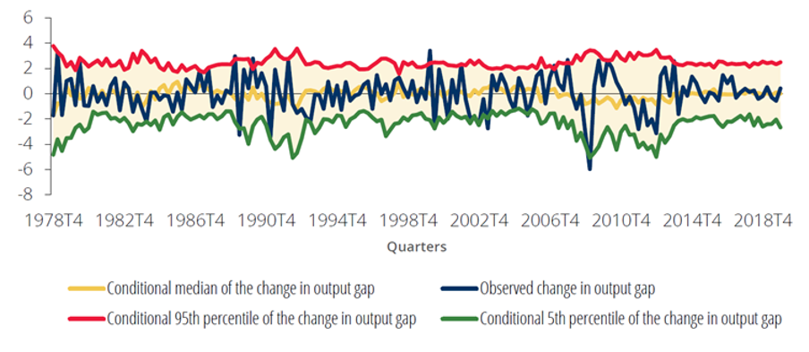
Note: results from one-quarter-ahead quantile regressions that include the current output gap change, inflation and the Country-Level Index of Financial Stress (CLIFS) as regressors. Source: Banco de Portugal, authors’ calculations.
Figure 2 indicates that the difference in volatility between the 5th and 95th percentiles of the estimated distribution of the output gap change is fully explained by the CLIFS, which is a measure of financial risk materialisation and a proxy of financial conditions dynamics in the regression. When the variable CLIFS increases by one-standard deviation, indicating a tightening of financial conditions, the estimated marginal effect on the lowest values of the output gap change decrease by 15 p.p. while it is not statistically significant in higher values. This result implies that high risk materialisation today, corresponding to tight financial conditions, has a more negative effect on the lowest values of the output gap change in one quarter compared to the rest of its values. The other variables in the regression are not significant for any percentile. In other words, the right-hand tail of the distribution of the output gap stays roughly constant, while the left-hand tail varies with financial conditions.
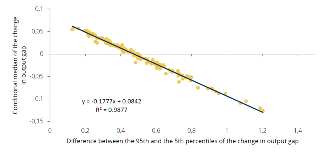
We can thus conclude that financial conditions, by driving the difference in volatility between the tails of the distribution of the output gap change, are responsible for the non-linear developments of the output gap change. An increasing volatility of the output gap change corresponds to higher probability of observing extreme negative output gap change realizations. Figure 3 shows that the volatility of the estimated distribution of the output gap change – measured as the difference between the estimated 95th and 5th percentiles – is negatively correlated with its conditional median. In other words, low realizations of the output gap change are associated with periods in which its extreme negative realizations are more likely to occur. The empirical results suggest overall that the output gap change volatility is not constant also for Portugal and that, similarly to the results from Adrian et al. (2020), this is due to financial conditions.
Figure 2. Marginal contributions to the output gap change
(percentage points)
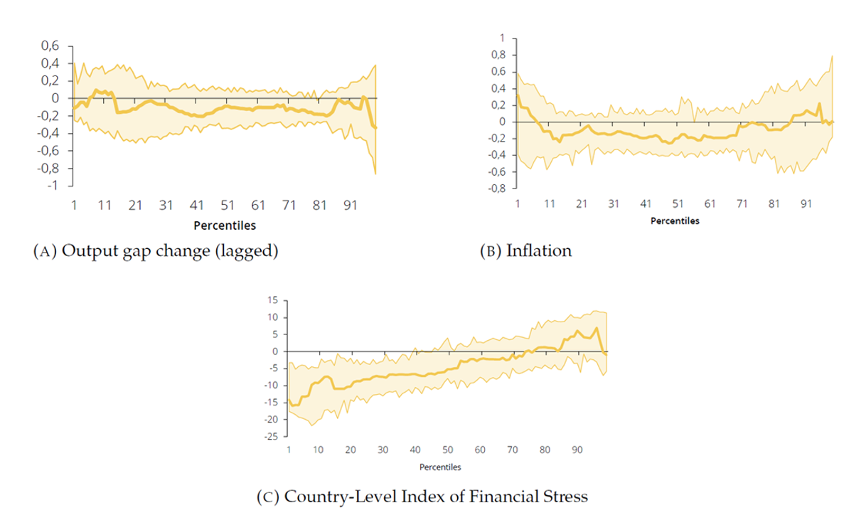
Note: results from one-quarter-ahead quantile regressions that include the current output gap change, inflation and the Country-Level Index of Financial Stress (CLIFS) as regressors. The shaded areas stand for 95% confidence intervals obtained using bootstrapping (xy-pair method) according to Davino et al. (2013). The estimated marginal effects are conditional on a one standard deviation increase holding constant all other regressors. Source: Banco de Portugal, authors’ calculations.
Figure 3. Correlation of the estimated one-quarter-ahead output gap change with its volatility
(percentage)
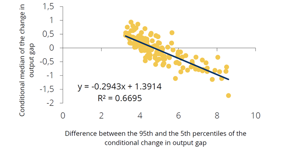
Note: results from one-quarter-ahead quantile regressions that include the current output gap change, inflation and the Country-Level Index of Financial Stress (CLIFS) as regressors. Source: Banco de Portugal, authors’ calculations.
The core novelty of the Adrian et al. (2020)’s paper is the specification of the non-constant volatility of the output gap (i.e., the vulnerability channel), which is modeled to depend on past financial conditions and past values of the output gap. These modeling choices are justified by the stylized facts reported in Section 2, where we show that financial conditions today negatively affect the output gap change volatility in one quarter, and that there is a (negative) correlation between the output gap change volatility and its conditional median.
The NKV model is an extension of a standard NK model that can be reduced to a three-equation system. The first equation is an IS curve, which models the combinations of the output gap and the interest rate that guarantee the general equilibrium in the real sector of the economy. The IS curve also includes a “financial accelerator” term, to account for the well-known amplification effects of financial developments on economic realizations. Loose (tight) financial conditions have a positive (negative) impact on economic growth. In addition, the IS curve includes an extra wedge to ensure that the variance of the shock to the equation is conditionally heteroskedastic, which depends on past values of financial conditions and the output gap, varying with past state variables. A Phillips curve summarizes the positive relationship between inflation and the output gap. Finally, a Taylor Rule defines a standard monetary policy where the policy interest rate depends on inflation and economic growth. The authors also assume current financial conditions to be dependent on contemporaneous and expected output gap, with current and expected positive economic developments being associated with looser financial conditions today. In the model, financial conditions depend indirectly on the interest rate through the IS curve, and this feature allows the risk-taking channel of monetary policy. This vulnerability feature enables intertemporal risk-taking dynamics, with low current economic volatility triggering higher leveraging and causing higher expected future volatility in the output gap.
The model is fitted to Portuguese data according to the existing literature on the estimation of DSGE models (Smets and Wouters 2003, 2007; An and Schorfheide 2007; Fernández-Villaverde and Rubio-Ramírez 2007).1 First, we estimate a subset of parameters for a linear version of the model, using pre-set standard values for the rest of them (chapter 3 of Galí 2008 textbook). Second, we estimate the non-linear parameters matching some Portuguese empirical moments. The following 1994-2019 time series are used as observables in the estimation: labour (hours), the Country-Level Index of Financial Stress (CLIFS), which is an indicator that comprises six, mainly market-based, financial stress measures that capture three financial market segments: equity markets, bond markets and foreign exchange markets (Duprey et al. 2015), the euro area shadow short-term interest rate (Krippner website, ljkmfa.com), year-on-year core inflation, the output gap, the output gap change, the expected output gap change, and the estimated volatility of the output gap change. The expected output gap change and the estimated volatility of the output gap change are obtained from the one-quarter-ahead quantile regression discussed in Section 2.
To compare the empirical results in Section 2 with those simulated by the model, we compute the median, the 5th and the 95th percentiles of the distribution of the output gap change, obtained by producing 200-quarter responses of the model to random supply-side, monetary-policy, and financial-conditions shocks. Figure 4 shows that the standard deviation of the 5th percentile of the output gap change is 2.12 times the standard deviation of the 95th percentile. Figure 5 shows that the volatility of the estimated distribution of the output gap change is negatively correlated with its conditional median. The NKV model estimated for Portugal is thus able to replicate the stylized facts reported in Section 2. We conclude that simulation results obtained from the NKV model for Portugal match well the empirical evidence from the quantile regressions.
The non-linearity in the realizations of the output gap is driven by the time-varying nature of volatility in the model. With the purpose of illustrating the importance of current and expected financial conditions for the future realizations of the output gap, we consider our baseline model specification with non-constant volatility (i.e. with the vulnerability channel) and a specification where the volatility of the output gap is kept constant (without the vulnerability channel).
We compute a 10000-period simulation of the two specifications, where state variables are randomly buffeted with supply-side, monetary-policy, and financial-conditions shocks.
Figure 6 indicates that the simulated distributions of the output gap and the output gap change obtained with the non-constant volatility specification are more asymmetric compared to the constant volatility specification, signalling that it is precisely the vulnerability channel of the model that is responsible for the non-linear realizations of the output gap. The more frequent positive values for the output gap change and the more frequent negative values for the output gap in the non-constant specification indicate that the economy changes more rapidly and is more likely to experience recessions when the financial conditions drive the output gap volatility.
Figure 4. Simulation of the changes in the output gap
(% deviation from the steady state)
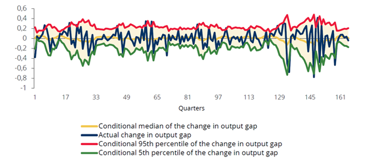
Note: the actual output gap change is the change computed in a benchmark simulation. Estimated percentiles are computed relative to the benchmark simulation. Source: Banco de Portugal, authors’ calculations.
Figure 5. Correlation of the simulated output gap change with its volatility
(% deviation from the steady state)
Note: estimated percentiles are computed relative to a benchmark simulation. Source: Banco de Portugal, authors’ calculations.
Figure 6. Simulated distributions – non-constant vs constant volatility
(probability)
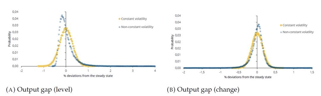
Source: Banco de Portugal, authors’ calculations.
In this study, we are also interested in observing the consequences of having more/less volatile financial conditions in the model, to get some insight into the impact of policies that may reduce their volatility. Given the introduction of the vulnerability channel in a standard NK model, we can model a scenario with more volatile financial conditions. We compute impulse response functions – with random shocks perturbating the model over a 10000-period simulation as in the previous exercise – for the variables of the baseline specification with non-constant volatility and for an alternative specification with non-constant volatility and more volatile financial conditions than in the baseline specification.
Figure 7 shows that the presence of more volatile financial conditions amplifies the intertemporal risk-taking dynamics in the model (panel in the left). In addition, the panel in the right shows that the simulated distribution of the output gap in the alternative specification with non-constant volatility and more volatile financial conditions is more volatile than in the baseline specification with non-constant volatility and less volatile financial conditions.
With more volatile financial conditions in fact, low volatility of the output gap today results in overall more volatile realizations of the output gap in the future compared to baseline specification with non-constant volatility. These dynamics translate into a more dispersed distribution of the output gap, with a higher probability of observing extreme values (positive and negative). The model in the specification with constant volatility is unable to capture this result, and for this reason, the non-constant volatility feature should be taken into account by policymakers.
Figure 7. Simulated distributions – non-constant vs constant volatility with more volatile financial conditions
(probability)
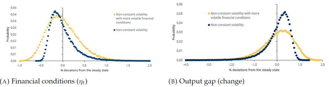
Source: Banco de Portugal, authors’ calculations
Some recent macroeconomic literature is raising awareness on the need for adapting existing – or developing new – structural methodological frameworks to understand how severe macroeconomic downturns could be in the case of extreme events. The NKV model proposed in Adrian et al. (2020) is a pioneer approach to include a financial vulnerability channel in a structural macroeconomic model and embodies a significant starting point to study the impact of non-linearities in these types of frameworks.
In the NKV model estimated for Portugal, we replicate the non-linearities which are evident in the data, with financial conditions affecting lower realizations more than higher realizations of the output gap change, thus driving its volatility. In addition, low realizations of the output gap change are associated with periods in which its extreme negative realizations are more likely to occur. The model highlights a crucial intertemporal risk trade-off faced by policymakers, as low volatility of the output gap today triggers excessive risk-taking and results in overall more volatile realizations of the output gap in the future. Our results show that reducing the volatility of financial conditions can alleviate the intertemporal risk-taking dynamics.
Although the NKV model is limited to a short-term perspective since it is specifically designed to match one-quarter-ahead dynamics, it constitutes an important added value for policymakers, as reproduces agents’ risk-taking intertemporal behaviour and the interaction of key macroeconomic variables, while including inflation and monetary policy. Therefore, this framework is useful to assess the financial stability implications of accommodative monetary policy, but also monetary policy rules that take into account financial stability risks throughout the financial cycle, by tightening to lean against the wind when cyclical systemic risk builds up and loosening to “clean” when systemic risk materialises. In turn, the model can also be extended to integrate macroprudential policy, which, alongside microprudential policy, is defined as the first line of defence against the build-up of financial stability risks. Macroprudential measures may be better suited to deal with intertemporal risk-taking trade-offs generated by accommodative monetary policy stance, because it is specifically designed to address the financial markets imperfections and externalities which cause them, complementing monetary policy actions, which is particularly relevant in a monetary union. Countercyclical macroprudential policy rules, such as the ones mimicking countercyclical capital buffers, could be assessed against the worsening of financial imbalances leading to higher capital buffers and resilience of the institutions. In this context, the effectiveness of these policy rules in reducing the medium-term financial stability risks created by monetary policy accommodation can be examined. Finally, the interactions between the two policy domains and their role in stabilising financial conditions can also be explored, complementing growth-at-risk empirical analysis to support policy decisions.
Adrian, Tobias, Nina Boyarchenko, and Domenico Giannone (2019). “Vulnerable Growth.” American Economic Review, 109(4), 1263–1289.
Adrian, Tobias, Fernando Duarte, Nellie Liang, and Pawel Zabczyk (2020). “NKV: A New Keynesian Model with Vulnerability.” AEA Papers and Proceedings, 110, 470–476.
Aikman, David, Kristina Bluwstein, and Sudipto Karmakar (2023). “A tail of three occasionally-binding constraints: a modelling approach to GDP-at-Risk.” Working paper 931, Bank of England.
Aikman, David, Jonathan Bridges, Sinem Hacioglu Hoke, Cian ONeill, and Akash Raja (2019). “Credit, capital and crises: a GDP-at-Risk approach.” Working paper 824, Bank of England.
An, Sungbae and Frank Schorfheide (2007). “Bayesian analysis of DSGE models.” Econometric Reviews, 26(2-4), 113–172.
Brownlees, Christian and André B.M. Souza (2021). “Backtesting global Growth-at-Risk.” Journal of Monetary Economics, 118, 312–330.
Carriero, Andrea, Todd E. Clark, and Massimiliano Marcellino (2024). “Capturing Macro-Economic Tail Risks with Bayesian Vector Autoregressions.” Journal of Money, Credit and Banking, 56(5), 1099–1127.
Cesa-Bianchi, Ambrogio and Emilio Fernandez-Corugedo (2018). “Uncertainty, Financial Frictions, and Nominal Rigidities: A Quantitative Investigation.” Journal of Money, Credit and Banking, 50, 603–636.
Christiano, Lawrence J., Roberto Motto, and Massimo Rostagno (2014). “Risk Shocks.” American Economic Review, 104(1), 27–65.
De Lorenzo Buratta, Ivan, Marina Feliciano, and Duarte Maia (2022a). “How Bad Can Financial Crises Be? A GDP Tail Risk Assessment for Portugal.” Working Paper Series 04, Banco de Portugal.
De Lorenzo Buratta, Ivan, Marina Feliciano, and Duarte Maia (2022b). “Mind the Build-up: Quantifying Tail Risks for Credit Growth in Portugal.” Working Paper Series 07, Banco de Portugal.
De Lorenzo Buratta, Ivan and Diana Lima (2025). “The vulnerability channel: assessing the impact of financial conditions on the output gap.” Economic Studies, Vol. XI, No. 4, Banco de Portugal. (Available at: https://www.bportugal.pt/sites/default/files/documents/2025-10/RE202512_EN.pdf )
Duprey, Thibaut, Benjamin Klaus, and Tuomas Peltonen (2015). “Dating systemic financial stress episodes in the EU countries.” Working Paper Series 1873, European Central Bank.
Fernández-Villaverde, Jesus and Juan F. Rubio-Ramírez (2007). “Estimating macroeconomic models: A likelihood approach.” Review of Economic Studies, 74(4), 1059–1087.
Galí, Jordi (2008). Introduction to Monetary Policy, Inflation, and the Business Cycle: An Introduction to the New Keynesian Framework. Princeton University Press.
Lang, Jan Hannes, Cosimo Izzo, Stephan Fahr, and Josef Ruzicka (2019). “Anticipating the bust: a new cyclical systemic risk indicator to assess the likelihood and severity of financial crises.” Occasional Paper Series 219, European Central Bank.
Montes-Galdón, Carlos, Viktors Ajevskis, František Brázdik, Pablo Garcia, William Gatt, Diana Lima, Kostas Mavromatis, Eva Ortega, Niki Papadopoulou, Ivan De Lorenzo Buratta, and Benedikt Kolb (2024). “Using structural models to understand macroeconomic tail risks.” Occasional Paper Series 357, European Central Bank.
Papadamou, Stephanos, Moise Sidiropoulos, and Aristea Vidra (2018). “A Taylor Rule for EU members. Does one rule fit to all EU member needs?” The Journal of Economic Asymmetries, 18, 1–1.
Passinhas, Joana and Ana Pereira (2023). “A macroprudential look into the risk-return framework of banks’ profitability.” Working Paper Series 03, Banco de Portugal.
Smets, Frank and Raf Wouters (2003). “An estimated dynamic stochastic general equilibrium model of the euro area.” Journal of the European Economic Association, 1(5), 1123–1175.
Smets, Frank and Raf Wouters (2007). “Shocks and frictions in US business cycles: A Bayesian DSGE approach.” American Economic Review, 97(3), 586–606.
This work was developed under the scope of the European Central Bank WGEM-WGF Expert Group on Macro-at-Risk, published as an ECB Occasional Paper “Using structural models to understand macroeconomic tail risks”. Special thanks to Leonardo Urrutia from Leipzig University (Institute for Theoretical Economics – Macroeconomics) for providing the codes and help regarding the estimation. This section follows his methodological approach.