In this paper we provide a cost-benefit analysis of the borrower-based measures implemented by the National Bank of Slovakia. DSTI measures affected mainly the riskiest borrowers with at most secondary education and lower income. Exemptions from DTI limits are provided mainly to borrowers with a higher volume of loans and higher education. LTV limits affected mainly younger borrowers up to 35 years old. The impact of respective measures was affected by front-loading, by the gradual tightening of the limits and by other legislative changes. The highest impact is estimated in 2019, when the volume of newly granted loans was lowered by 17% due to the measures. The estimated impact on residential real estate prices is relatively mild. During adverse developments, DSTI limits affect the probability of default, LTV limits affect more loss given default and DTI limits impact mainly the volume of newly granted loans. This was visible also during the coronavirus pandemic, when DSTI measures have helped to mitigate households’ credit risk.
The NBS has been implementing borrower-based measures (BBMs) since end-2014 for several reasons. First, the annual growth rate of retail loans was for years the highest among all EU countries. Second, since 2015, this trend has been complemented also by increasing residential real estate prices. Finally, the increasing volume of loans translated into growing households’ indebtedness. The latter was identified as one of the main systemic risks for the Slovak banking sector. These different reasons have led to different goals aimed by respective phases of implementation and tightening of BBMs. An overview of these goals is described in Harrison et al. (2018).
Different limits have been imposed. In 2014, a Loan-to-Value (LTV) and Debt service-to-Income (DSTI) limit, a maximum maturity for housing as well as consumer loans and an interest rate shock were introduced in the form of a recommendation. Since 2017 the recommendation has been transformed into binding legislation. LTV and DSTI limits have been gradually tightened and a Debt-to-Income (DTI) limit was implemented in mid-2018. As of end-2019, the LTV limit was 90%, 20% of new loans could be granted with LTV between 80% and 90%. The DSTI limit was 80%. The DTI limit was 8, 10% of new loans could be granted with higher DTI, with half of this exception being dedicated to young borrowers. The DSTI limit was gradually tightened in 2020 to 60%, but as the development of loans in 2020 was significantly affected by the corona pandemics, we are analysing the impact of borrower-based measures only up to end-2019. More details about the setting of BBMs can be found in Cesnak et al. (2021).
There is a growing literature discussing the impact of BBMs. On the positive side, limits prevent excessive credit growth or the excessive growth of households’ indebtedness. Furthermore, they mitigate adverse impact on banks and debtors in case of negative shock, when cumulated risks can materialise. Cassidy and Hallissey (2016) or Gross and Población (2017) concluded that BBMs are efficient in mitigating losses stemming from the retail loan portfolio by decreasing the probability of default as well as the loss given default. Empirical analysis also confirms a link between BBMs and credit growth or real estate prices. Richter et al. (2018), Vandenbussche et al. (2015), Ahuja and Nabar (2011) or Igan and Kang (2011) shows, on a relatively large sample of countries, that imposing LTV and/or DTI limits reduce housing loans growth and consequently also real estate price growth. Kuttner and Shim (2012) concluded that tightening of DSTI affects more the volume of loans while tightening of LTV affects more real estate prices.
The implementation of BMMs can, however, have some unintended consequences as well. Some of these consequences have already been discussed by other central banks having implemented such measures (see e.g. Cassidy and Hallissey, 2016). In case of LTV and LTI limits applied on housing loans the following points are discussed:
As some of these points are addressed directly by the design of the measures implemented by the NBS, we are focusing on the following points:
The identification of the group of clients affected the most by the respective measures is based on the change in the distribution of loans, econometric analysis (logit regressions) and machine learning techniques (decision trees). For further details, see Cesnak et al. (2021). Our main findings are the following:
Using the method of stochastic frontier, it is possible to estimate the maximum attainable amount of loan based on the assumed input parameters at the time of loan origination. Not all the loans are granted at the maximum possible amount due to differences across regions, banks, and demand, while this method enables us to estimate this “inefficiency”. The assessment in this part focuses on housing loans. We estimate the attainable amount of loan and the inefficiency term using income, borrowers’ own capital, age, interest rate and the collateral as explanatory variables and controlling for region and bank effects.
Income is having a positive impact on the production function and the coefficient for the collateral is also positive and close to one. The maximum amount of loan, or credit available, is estimated practically as the value of collateral minus own funds. If there are two loans with the same value of collateral, the larger loan having higher LTV is estimated to be more expensive, which is expressed by the positive coefficient for the interest rate. The inefficiency term is decreasing by increasing income and collateral and increasing by increasing own capital.
When estimating the production function and the inefficiency term on a yearly basis or in different periods with less and more tight BBM limits, we find that loans have been gradually granted closer to their theoretical maximum amount. This could be a consequence of the impact of BBMs on the maximum credit available and also the reaction of banks allowing for some clients to draw a higher amount of loan compared to the period with no BBMs.
To estimate the impact of the measures on the volume of newly granted loans, we assume that without these measures the distribution of loans would have remained unchanged compared to the last year preceding the implementation of the respective measures2. We estimate an upper and a lower bound of the possible impact and also estimate a more realistic potential impact of the limits. For the upper bound, i.e. the less restrictive estimation, we assume all households potentially asking for a loan exceeding a given limit asked for a loan exactly at the consecutive limit3. For the lower bound, we assume none of the households potentially asking for a loan exceeding a given limit asked for a loan after the limit was implemented.
Figure 1: Estimating the impact of tightening on the volume of new loans – scheme
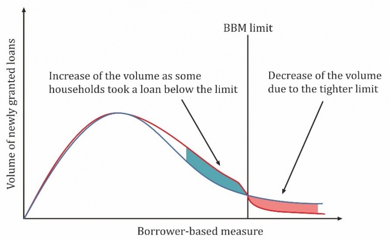
To estimate the potential impact, we consider the change in the distribution of the newly granted loans not just above the imposed limit but also under. Above the limit, we consider the possible decrease of the volume of newly granted loans due to the imposed limit (red area on Figure 1). Under the limit, we consider the potential increase of the volume of new loans as some households potentially asking for a loan above the limit could have taken a loan just below the newly imposed limit (blue area on Figure 1). The overall impact is then the net change in the volume of newly granted loans.
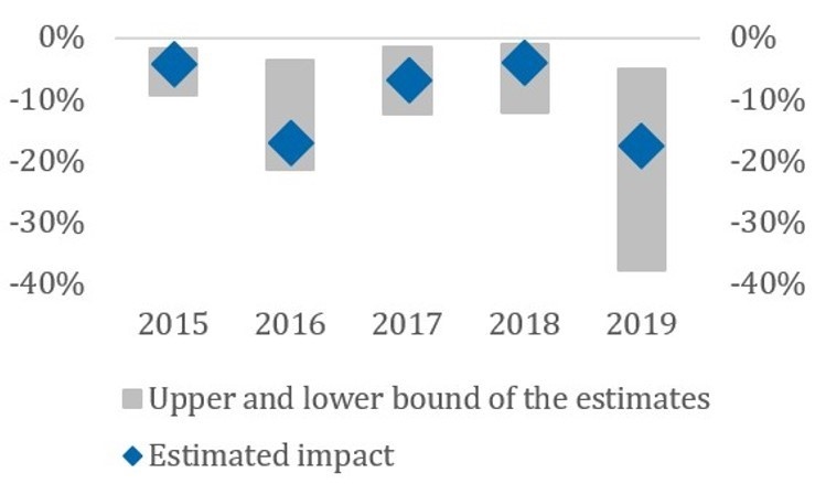
The difference between the impact on overall retail loans and on retail housing loans is relatively small due to the high share of the volume of newly granted housing loans in the volume of newly granted retail loans. The highest impact is in 2016 and in 2019, when the impact of DTI and DSTI limits was the highest. However, in 2016 a new legislation was introduced4, affecting refinancing with a possible consequent impact also on the estimates for this year. In 2019, we estimate that the volume of newly granted loans was lowered by 17% and the volume of newly granted housing loans by 19% by the measures. It means that with the measures in place, the volume of retail loans is lower by 17% compared to the possible figures in this year without the measures. In 2019, the DSTI limit had the highest impact on this decrease, followed by LTV and then by the DTI limit.
Figure 2: Overall estimated impact of limits on the volume of newly granted loans
| Impact on retail loans | Impact on retail housing loans |
 |
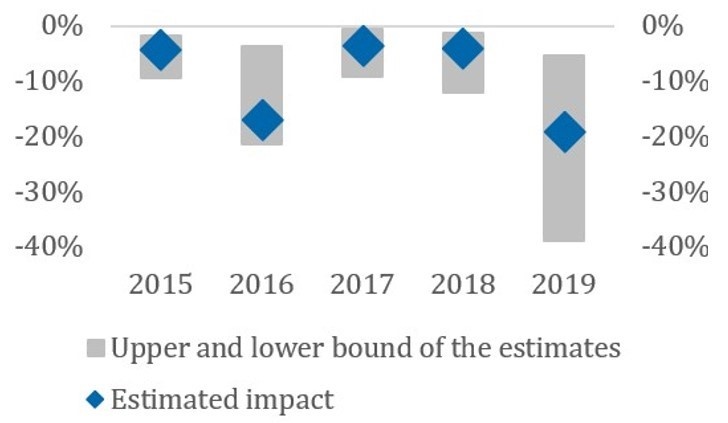 |
Source: NBS.
Note: Chart shows percentage changes in the volume of estimated newly granted loans.
We estimate both a quantitative and qualitative impact of the BBMs on the residential real estate prices. To estimate the qualitative impact, we estimate the maximum attainable value of a housing loan for a given household using similar methodology as described in Cesnak and Klacso (2021). This enables us to directly account for the impact of BBMs on the attainable amount of loan.
Until 2019, implemented BBMs were not constraining significantly for a household with average wage using average interest rates on housing and consumer loans, as well as average wages. It means that the maximum attainable loan for such a household exceeded average residential real estate prices. Gradual tightening of BBMs decreased loan availability as well. At the end of 2019, the estimated attainable amount of loan for some selected type of households, mainly for those without enough capital of their own, was the closest to average residential real estate prices within the last 10 years.
Based on the predicted development of loan availability, the impact of BBMs should increase, resulting in a significant decrease of the amount of loan attainable compared to the real estate prices. Potential borrowers without enough capital of their own can be the most affected section of potential borrowers.
Within the qualitative impact, we use error-correction models to estimate the long-run relationship between residential real estate prices and the volume of newly granted housing loans. Based on the estimations, in the long run about 2% to 20% of the change in the volume of housing loans is transmitted into changes in real estate prices. Based on the estimated change in the volume of newly granted housing loans after the implementation of BBMs we can, thus estimate the potential change in house prices. In general, the estimated impact is relatively mild. The estimated decrease of the volume of newly granted housing loans in 2019 at the level of 19% is transmitted in the long run to the decrease of real estate prices at the level of 0.5% – 4.5%. Based on the estimated adjustment coefficients, the changes are transmitted within 5 to 9 quarters.
The efficiency of macroprudential policies, including BBMs, should be measured during times of increased stress. The efficiency of BBMs during adverse development is described in Jurča et al. (2020). Different measures impact the cumulation of systemic risks caused by the excessive loan growth and the consequent impact on banks via different channels. While DSTI limits affect the probability of default, LTV limits affect more loss given default. DTI limits impact mainly the volume of newly granted loans. The analysis confirmed also that the timely implementation of BBMs is an efficient tool for increasing the resilience of the banking sector. Last but not least, the most efficient way of curbing the cumulation of systemic risks is the combined implementation of different measures, as they are complementary to each other.
The COVID-19 pandemic is the first negative shock since BBMs have been implemented impacting the real economy and indebted population. To mitigate the impact of the virus, the government implemented several measures during 2020. For households, one of the key measures was the possible loan payment deferral for 6 to 9 months. Due to this measure, there was basically no default of retail loans in 2020. However, the analysis of households asking for this deferral can help to identify households impacted by the pandemic the most and to assess BBMs. The characteristics of households asking for deferral until August 2020 were studied in Cupa k et al. (2020). A higher decrease of income due to the pandemic increases the probability of a household asking for deferral. However, higher pre-crisis DSTI also increased this probability, as even a smaller decrease of income could result in a situation where a given household was not able to repay its loans. This outcome confirms the importance of the proper calibration of the DSTI limit.
Ahuja, A. and Nabar, M. (2011). Safeguarding Banks and Containing Property Booms: Cross-Country Evidence on Macroprudential Policies and Lessons from Hong Kong SAR. IMF Working Paper, WP/11/284.
Cassidy, M. and Hallissey, N. (2016). The Introduction of Macroprudential Measures for the Irish Mortgage Market. The Economic and Social Review, 47(2), pp. 271-297.
Cesnak, M., Cupák, A., Jurašeková Kucserová, J., Jurča, P., Klacso, J., Košútová, A., Moravčík, A. and Šuster, M. (2020). Vplyv koronakrízy na finančnú situáciu a očakávania zadlžených domácností. NBS Occasional paper, 3/2020.
Cesnak, M. and Klacso, J. (2021). Assessing real estate prices in Slovakia – a structural approach. NBS Working paper, 3/2021.
Cesnak, M., Klacso, J. and Vasiľ, R. (2021). Analysis of the Impact of Borrower-Based Measures. NBS Occasional paper, 3/2021.
Gross, M. and Población, J. (2017). Assessing the Efficacy of Borrower-Based Macroprudential Policy Using an Integrated Micro-Macro Model for European Households. Economic Modelling, 61, pp. 510-528.
Harrison, O., Jurča, P., Rychtárik, Š. and Yackovlev, I. (2018). Credit Growth and Macroprudential Policies in the Slovak Republic. V: IMF Country Report, 18(242). Slovak Republic.
Igan, D. and Kang, H. (2011). Do Loan-to-Value and Debt-to-Income Limits Work? Evidence from Korea. IMF Working Paper, WP/11/297.
Kuttner, K. and Shim, I. (2012). Taming the Real Estate Beast: The Effects of Monetary and Macroprudential Policies on Housing Prices and Credit. RBA Annual Conference, in: Alexandra Heath a Frank Packer a Callan Windsor, Property Markets and Financial Stability, Reserve Bank of Australia.
Richter, B., Schularick, M. and Shim, I. (2018). The Costs of Macroprudential Policy. NBER Working paper 24989.
Vandenbussche, J., Vogel, U. and Detragiache, E. (2015). Macroprudential Policies and Housing Prices: A New Database and Empirical Evidence for Central, Eastern, and Southeastern Europe. Journal of Money, Credit and Banking, 47(1), pp. 343-377.
Data are available for regularly received net income of the borrowers.
For the DSTI limit, we use 2015 as the reference year, for DTI 2017 and for LTV 2014.
E.g. if a household asked for a loan in 2018, the DSTI limit was 80%. If the household planned to ask for a loan exceeding this limit, we assume it took a loan with a DSTI being exactly 80%.
The fee for refinancing a loan was significantly lowered, to at most 1% of the outstanding amount of the refinanced loan.