A high-dimensional GDP-at-risk and Inflation-at-risk for the euro area

Abstract
GDP-at-risk and Inflation-at-risk are standard measures of tail risk in modern macroeconometrics, adapted from tools originally developed in the financial risk management literature. In this work, these indicators are estimated for the euro area and its Member States by leveraging a high-dimensional dataset in the construction of time-varying conditional distributions of GDP growth and inflation. The distributions obtained at country level are used to assess how the synchrony of euro-area countries’ business cycles has evolved since the introduction of the euro. The results indicate significant asymmetries in the balance between upside and downside risks for both GDP and inflation, and a persistently weak synchrony for the left tails of GDP growth distributions during episodes of crisis.

Tail risk indicators as a tool to deal with uncertainty

Uncertainty on the future state of the economy is often managed by complementing point forecasts with probability distributions of the variables of interest, conditional on a series of financial and economic indicators. The tails of these distributions, capturing outcomes in worst-case scenarios, are especially informative and under scrutiny in turning points of the business cycle. The recurrence of periods of macroeconomics stress has fostered a large literature on this topic, which has borrowed and adapted modelling approaches from financial risk management as the Value-at-risk (Cecchetti (2006, 2008), Adrian, Boyarchenko, and Giannone (2019), Aikman et al. (2019) among others). Previous studies on the Euro Area (Figueres and Jarociński (2020), Chavleishvili and Kremer (2023), Szendrei and Varga (2023), Chavleishvili and Manganelli (2024) among others) have found a non-linear relationship between GDP growth and financial stress indicators, as well as asymmetries between the tails of the GDP growth conditional distribution.

Conditional distributions of GDP growth and inflation in the Euro Area

In this study, I estimate conditional distributions of GDP growth and inflation and construct measures of their tail risks for the Euro Area (EA) and its member countries. The estimated distributions are based on factors extracted from a large dataset covering macroeconomic and financial variables for the Euro Area and its main member states (Barigozzi et al. (2024)), using a partial quantile regression (PQR) approach. Factors obtained by PQR (Giglio et al. (2016)) condense the most relevant information for a target variable at a specific quantile, thus exploiting large information sets and avoiding strong assumptions on the indicators to be included in the conditioning set.1

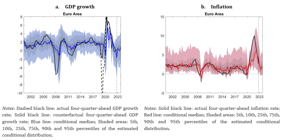
The tails of the conditional distribution of GDP (Figure 1a) are strongly asymmetric: while the right tail, measuring unexpected growth, hovers around 3-4 percent across the whole sample, the left tail – measuring the GDP-at-risk – varies significantly in time and falls drastically during crises.2 Dispersion tends to increase when the median shrinks, hinting at a negative relationship between the first and the second moment of the distribution. This feature of the distribution characterizes recessions as periods of combined economic downturn and higher uncertainty.3 For what concerns prices, the right tail of the conditional distribution (Figure 1b), a measure of inflation-at-risk, is the most volatile part of the distribution, although the asymmetry is less pronounced than that observed for economic growth.4 The dispersion of the distribution increases when inflation is higher: high inflation risks, unlike deflation risks, are associated to higher uncertainty on future price growth.5

Figure 1. Conditional distributions, Euro Area (percentage points)

The conditional distributions of GDP growth and inflation can be considered jointly, so to evaluate the relationship between the two variables in different parts of their density functions. In the panels of Figure 2, each observation represents a pair of (y, π) conditional tail quantiles in a quarter. Considering the two variables on the same tail allows to interpret the point clouds as a conditional aggregate supply curve, evaluated at different points of the distributions.6 The curve outlined by conditional quantiles appears substantially flat on the left tail (Figure 2a), suggesting that positive demand shocks are unlikely to affect prices during times of weak economic activity. Conversely, the curve becomes steeper on the right tail (Figure 2b): when output growth is close to its potential, or in periods of high inflation, expansionary demand shocks would translate into price increases, with very limited effects on economic activity.

Figure 2. Conditional aggregate supply curve at different quantiles, Euro Area (percentage points)

Assessing macroeconomic synchrony at the quantiles

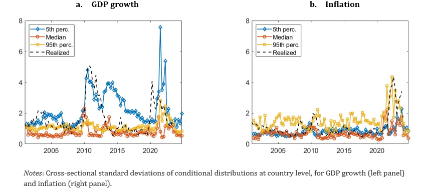
The conditional distributions of GDP growth and inflation estimated for the main EA countries lead to similar conclusions on the asymmetry between tails and the slope of conditional AS curves. These distributions can be also used to compute a measure of time-varying synchrony between economic cycles across the EA, with the advantage over indices based on realized outcomes of capturing synchrony on the whole distribution. The cross-sectional dispersion of the member states’ GDP growth distributions7 (Figure 3a) is quite low at the median the whole sample8; similarly, the right tails of the distributions are quite synchronized throughout the period. On the contrary, the synchrony of left tails varies significantly across time, with very large spikes in periods of distress, after which it reverts quite slowly to the lower levels observed before crises. From a longer term perspective, there are little signs of convergence of left tails, suggesting small improvements in the synchronization of economic cycles in bad times.

For inflation (Figure 3b), the average dispersion of the right tails is higher in comparison to the median and the lower percentiles. The dispersion of the right tail of the inflation distribution varies in time less than the one computed on the GDP-at-risk, and returns quite quickly to lower levels, suggesting that the degree of divergence during times of upside risks to prices increases significantly less than downwards risks to economic activity; furthermore, the dispersion of the distributions is quite limited on the whole distribution, indicating a high and stable level of synchronization of price growth in the EA, reached already before the introduction of the common currency.

Figure 3. Conditional cross-sectional standard deviation at different quantiles (percentage points)

Concluding remarks

This policy brief has presented estimates of the GDP-at-Risk and Inflation-at-risk for the Euro Area and its member states obtained from the information provided by a large dataset. Results indicate strong asymmetries in the GDP growth distribution, which displays fatter and volatile left tails in contrast with steadier right tails, and a higher uncertainty around outcomes during recessions. Opposite – but minor in extent – asymmetries are found also in the inflation distribution, which displays fatter and more volatile right tails, while remaining fairly stable on its lower quantiles in the whole sample. For what concerns synchrony between countries, results lead to mixed conclusions. The persistently low synchrony of GDP growth left tails during crises casts some doubts on the convergence of economic cycles; on the other hand, the short deviations of the conditional distribution from target levels of inflation indicate a good level of synchrony of upside risks to inflation across countries in the euro area, at least in the analysed sample, characterized by positive shocks to the price level that hit member states quite symmetrically.