We introduce the concept of cumulative wage gap – meaning the cumulative gap between the current wage and a peak reference wage value in the past. After a crisis, people relate to their peak gains in the past rather than to uncertain future gains. The shape of the post-crisis Phillips Curve expresses the theoretical assumption that the inflation rate stays below its target until the cumulative real wage gap closes, and that it increases above its target when the cumulative real wage gap becomes positive. We confirm our hypothesis using data for 35 OECD countries for the period 1990-2017. Inflation depends on the cumulative wage gap: it does not increase close to or above its target level until the cumulative real wage gap is closed. For Phillips Curve to work, the loss of welfare from a negative cumulative real wage gap has to be fully compensated first – as a stock measure, not as a flow.
The Phillips Curve has failed to explain why inflation has been subdued in the post-crisis years. It is probably the greatest mystery of the economic science in the last decade: where has the Phillips Curve gone? There are multiple references to the fact that the Phillips Curve has flattened over the last decade, if not earlier – Forder (2014), Praet (2016), Leduc and Wilson (2017), Carney (2017), Cunliffe (2017), Murphy (2018), Bullard (2018). The flattened Phillips Curve and the lesser link between inflation and unemployment, inflation and output gaps, or inflation and wages, have multiple explanations. As presented in international literature, some of these explanations are: de-anchoring inflationary expectations, the labor market slack, a lower natural rate of unemployment, changes in expectations regarding the real pay growth, the decoupling between growth and inflation, the role of global value chains in keeping prices down, the role of migration in keeping wages down in the countries of destination, among others. While there is some truth in each and every of them, no convincing explanation has been successfully suggested so far.
This is why three major changes are needed to the Phillips curve.
First, we should work with observable variables only. The built-in problem with econometric models which use non-observable variables is that they tend to under-perform in bad times. The output gap depends on potential GDP, which can be revised retroactively. Moreover, an economy can grow above its potential without being at full employment. Any measure of unemployment is controversial, given the impact of insufficiently accounted factors such as the underground economy, migration, inactivity, part-time employment. A non-observable measure of unemployment, like non-accelerating rate of unemployment (NAIRU), is even more questionable. Central Banks should not rest their decisions solely on non-observable variables. Therefore, we simplify the model by dropping the non-observable variables. Instead, we choose to use observable variables only. Wage is a measurable, reliable, accounted for, and comparable indicator. Hence, we focus on a wage Phillips Curve where consumer prices inflation rate is explained by the difference between past wages and current wages.
Second, we make a fundamental change of paradigm from flow to stock. Consumers’ behavior, which influences inflation, is usually overlooked in econometric models. To account for it, we introduce the concept of cumulative wage gap – meaning the cumulative gap between current wage and a peak reference wage value in the past. Stock is more relevant than flow because people have a strong preference which is their previous income levels. People do not spend as much as before when their wage drops, and they spend more if they have higher wages. While this is intuitive and apparently well explained, everything is related to wage flows and to wage dynamics. We hold that we should account for the stock as well, meaning the cumulative gap between current levels and past reference levels of income. Our hypothesis is that current consumption depends on the stock of income: people will not spend more until a negative cumulative wage gap closes, or, put differently, until they recover everything that they lost during a crisis.
Third, we allow for the Phillips Curve to be time-dependent: it moves over time, and it is absolutely normal to do so. Reference wage values, social preferences, jobs’ characteristics, skills’ endowments and even Central Banks’ targets – they all change over time. Therefore, the impact of cumulative wage gaps on inflation varies in different time periods. In fact, even Phillips (1958) stated that his hypothesis is not supported in or immediately after exceptional years (he referred to war years, when import prices rose rapidly enough to initiate a wage-price spiral).
Wages, the most important source of income for most households around the globe, stand at the basis of any consumption theory. The main problem with the prevailing consumption theories (Keynes’ consumption function (1936), Modigliani’s life-cycle hypothesis (1966) and Friedman’s permanent income hypothesis (1957)) is their long-term approach. This puts them at odds with our rather short and medium-term perspective on inflation, especially in times of crisis. Policy-makers cannot wait for market forces to play their role in the long-run. They need to act now and in order to do so they need a good explanation of inflation developments in the short and medium run.
We hold that the permanent income hypothesis is fundamentally flawed in times of crisis given the uncertainty of future income. The only certain reference value lies in the past, not in the future: this is why current consumption is influenced by past income.
Our approach is closer to Duesenberry (1952), who introduced relative income instead of the rate of change of income as the explanation of the differences in saving at the same level of income. He referred to the influence of past living standard on current consumption. Saving depends, he wrote, on the level of current income relative to higher incomes in previous years. However, he stopped short of calling a wage gap or of analyzing the influence his consumption and saving theory may have on inflation.
Our work starts from the assumption that a recession is a game – changer. In a recession, the transitory component of income becomes negative not only for one person or for a small group, but for the national or global economy. This makes it very difficult to predict future income. In a crisis, the only certain reference for wage earners is in their past. Retirement savings and linear employment prospects are uncertain. People relate to their peak gains in the not so distant past rather than to their uncertain future gains.
We assume that people judge their consumption decisions based on the relation between their current wages and their past wages, adjusted for inflation. Current consumption does not depend only on current income and future expectations, but also on past income. This is why we introduce the concept of cumulative wage gap – meaning the cumulative gap between current wage and a peak reference wage value in the past.
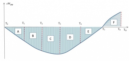
A theoretical graphical representation of the cumulative real wage gap for a six-period model (for simplicity reasons) is shown in Figure 1. We assume that the real wage is at a peak at T0, then it decreases until T2, then it starts to recover and it becomes positive between T3 and T4 and then it continues to grow until T6. At time T1, when real wage drops relative to its peak value, the cumulative real wage gap is the area A. At time T2, when real wage drops even further, the cumulative real wage gap is the sum of areas A and B. At time T3, when the real wage starts to increase, but as it remains below the peak value, the cumulative real wage gap further deepens (A+B+C). At time T4, when the real wage increases above the peak reference value, the cumulative real wage gap starts to shrink (A+B+C+D). The growth of real wage makes the cumulative real wage gap to close at time T5 (A+B+C+D+E) and to enter into the positive territory at time T6 (A+B+C+D+E+F).
Figure 1. The cumulative real wage gap, six-period model
Source: the author
Note: Area A is the cumulative real wage gap between T1 and T0, area B is the cumulative real wage gap between T2 and T1, area C is the cumulative real wage gap between T3 and T2, area D is the cumulative real wage gap between T4 and T3, area E is the cumulative real wage gap between T5 and T4 and area F is the cumulative real wage gap between T6 and T5.
It is important to understand the difference between stock and flow. For example, at T0 the real wage is at a peak, but as the real wage starts to drop afterwards, the cumulative wage gap is 0. At T4, policy-makers believe that they fuelled consumption because real wage is higher than it was initially at T0. However, the stock approach holds that the cumulative wage gap is still negative at T4 and the consumers” behaviour would not change until after T5 when the cumulative wage gap closes.
The cumulative real wage gap is the explanatory variable in our new Phillips Curve. The dependent variable is the inflation gap, which refers to the gap between inflation and the inflation target (or, in the absence of a target, an average value of inflation over a longer time-span).
Inflation gap is a more relevant variable for policy makers than the inflation rate because it puts inflation in relation to a desired level. A negative inflation gap means more demand-side measures are needed. A positive inflation gap means that the risk of overshooting is already present and policy tightening is required. For inflation, the reference point is not in the past – but it is rather a normative value, commonly agreed to be desirable for a given society at a given point in time.
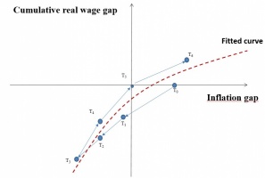
The shape of the post-crisis Phillips Curve expresses the theoretical assumption that the inflation rate stays below its target until the cumulative real wage gap closes, and that it increases above its target when the cumulative real wage gap becomes positive. The graphical representation assumes different slopes before and after closing the cumulative real wage gap. A sharper slope after closing the cumulative real wage gap means that the same amount of a cumulative real wage gap leads to less inflation as the cumulative gap is negative, and to more inflation as the cumulative gap turns positive.
Figure 2. The post-crisis Phillips Curve
Source: the author
At time T0, at the peak value of real wage, we assume that inflation rate is above the central bank’s inflation target, given the inflationary pressures caused by high wages. Therefore, inflation gap at time T0 is positive. As wages enter an adjustment phase, inflationary pressures fade away and inflation rate declines. Inflation gap turns negative and reaches a minimum at time T3, the same as the cumulative real wage gap. As wages resume growth, inflation rate starts rising, but it remains subdued, below the central bank’s inflation target, until time T5, when the cumulative real wage gap is closed. Afterwards, wages continue to increase and the wage gap widens in the positive territory. Consequently, inflationary pressures strengthen, pushing up the inflation rate above the central bank’s inflation target at time T6.
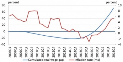
The initial source of inspiration for this stock-based approach of the post-crisis Phillips Curve was the case of Romania. Following a long deflationary trend inflation surged unexpectedly in the second half of 2017 from negative rates to 3.3 per cent at year-end 2017, and as high as 5.4 per cent in May 2018. Figure 3 shows the correlation between inflation and the cumulative wage gap. Austerity policies in 2010 led to nominal wage cuts. While nominal and even real wages were restored at their pre-2010 level as early as by 2013, the cumulative real wage gap only closed at the beginning of 2017. In this interval, minimum wage more than doubled, with only marginal impact on inflation (Heemskerk, Voinea, Cojocaru, 2018). After the cumulative wage gap closed, inflation surged.
Being encouraged by this empirical evidence, we tested the cumulative wage gap hypothesis for all OECD countries (except for Turkey, due to lack of data) over the period 1990-2017.
Figure 3. Cumulative wage gap and inflation in Romania, 2008 – 2018
Source: the author
The year T0 is the peak year. We define a wage adjustment episode the adjustment in real wages that follows after the peak year. For each wage adjustment episode in a country, the data sample starts at year T0 and it ends when a new peak is detected. If the cumulative wage gap has not been closed, then we consider a new peak as part of the same adjustment episode.
In the analysed period, there were three historical episodes of wage adjustments. Data shows that the cumulative real wage gap was closed in all countries which experienced the first wage adjustment episode, with the exception of two countries (Japan and Korea). In the case of the second wage adjustment episode, the cumulative real wage gap has not yet been closed, with the exception of other two countries (Mexico and Latvia). These latter two countries entered a new wage adjustment episode, the third one.
For simplicity reasons, the wage adjustment episodes are numbered with reference to the time periods and not to the country-specific episodes. We considered as the first wage adjustment episode any episode which started in the last decade of last century (1990-1999) and the second wage adjustment episode any episode which started after the year 2000.
Peak years are country-specific; hence they are not the same in all countries. This means that the first wage adjustment episode may have lasted 7 years in Italy, 8 years in Germany and France, 9 years in US, 20 years in Korea or 28 years (and counting) in Japan. Of the 35 countries analysed, 21 countries experienced the first historical episode of wage adjustments, 33 countries experienced the second historical episode of wage adjustments and only 2 countries experienced the third historical episode of wage adjustments.
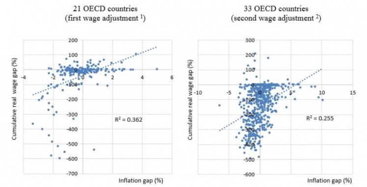
The graphical representation of our results is shown in Figure 4.
Figure 4. Post-crisis Phillips Curve for OECD countries
Source: the author
Notes: 1 Period 1993-2000 for AUS, AUT, BEL, DNK, FIN, FRA, DEU, IRL, LUX, NLD, NZL, CHE, GBR; 1994-2000 for ISL, ITA, NOR, ESP, SWE; 1990-2017 for JPN; 1998-2017 for KOR, 1989-1998 for USA.
2 Period 2001-2017 for AUS, AUT, BEL, CZE, DNK, FIN, FRA, DEU, HUN, ISL, IRL, ITA, LUX, LTU, NLD, NOR, NZL, PRT, SVK, SVN, ESP, SWE, CHE, GBR; 2002-2017 for CAN, EST, GRC, ISR, POL; 2003-2017 for CHL; 2001-2006 for LTV; 2004-2008 for MEX; 1999-2017 for USA.
Data sources for wages and inflation are the OECD and the FRED databases (for US), annual data. We transformed the average annual wage into local currency for ensuring comparability with the inflation rate, which reflects changes in local prices. Data sources for the inflation target of central banks are from the respective central banks’ websites. If a central bank targets a corridor rather than a level of the inflation rate, then the mid-point of the target band is considered.
The results are statistically significant and with the expected sign for the first two wage adjustment episodes. For the third wage adjustment episode, the sign of the relationship is as predicted, but the number of observations is too limited to have statistical significance.
The theoretical model is confirmed. The cumulative wage gap explains more than one third of the inflation gap in the first wage adjustment episode and more than one fifth of it in the second adjustment episode.
When aggregated for all OECD countries (Table 1), the estimated slopes of the post-crisis Phillips Curve are statistically significant at the 5% level for the first wage adjustment episode, and at the 1% level for the second wage adjustment episode. The coefficients’ sign is positive, in line with the theoretical assumptions.
Table 1. Estimated slopes, aggregated data, panel estimation with country fixed effects, log-normalized
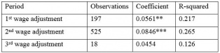
Source: the author
The results show that an increase/decrease of the cumulative real wage gap by 10% led inflation gap to rise/deepen by 0.561% during the first wage adjustment episode, by 0.846% during the second wage adjustment episode and by 0.454% during the third wage adjustment episode.
For the first wage adjustment episode, out of 21 countries, 8 of them have positive and statistically significant coefficients; other 7 countries have positive but not statistically significant coefficients, while the remaining 6 countries have negative but not statistically significant coefficients. The cumulative wage gap explains more than 60% of the inflation gap in Iceland, about two thirds of the inflation gap in the US and Ireland, more than half the inflation gap in Finland and Switzerland, close to half of the inflation gap in Netherlands. It even explains almost one quarter of the inflation gap in Korea, despite the fact that this country has not closed the first wage adjustment episode yet.
For the second wage adjustment episode, out of 33 countries, 16 of them have positive and statistically significant coefficients; other 9 countries have positive but not statistically significant coefficients, while the remaining 8 countries have negative coefficients, out of which only 2 are statistically significant. The cumulative wage gap, which in most cases has not been closed yet, explains more than 60% of the inflation gap in Slovenia and Slovak Republic, between 40% and 60% of the inflation gap in Greece, Italy, Portugal, and Spain, and between 20% and 40% of the inflation gap in Australia, Canada, Denmark, France, Hungary, Ireland, Netherlands, New Zeeland, Switzerland and United States.
We also estimated the slope of the post-crisis Phillips Curve before and after the cumulative real wage gap was closed (Table 2).
Table 2. Estimated slopes, before and after closing the cumulative wage gap,
panel estimation with country fixed effects, log-normalized
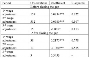
Source: the author
For the first wage adjustment episode, the results show that a fall of the cumulative real wage gap by 10% corresponds to a decline of the inflation gap by 0.9%. On the other hand, a 10% increase of the cumulative real wage gap after closes leads to an increased inflation gap by 2.2%. This confirms the theoretical prediction that there is a break in the slope of the curve, as the coefficients are higher after the cumulative wage gap closes than before this happens. For the second wage adjustment episode, the number of observations is too small to have a meaningful conclusion, since most countries have not yet closed the cumulative wage gap.
Bottom-line, inflation depends on the cumulative wage gap: it does not increase close to or above its target level until the cumulative real wage gap is closed. For Phillips Curve to work, the loss of welfare from a negative cumulative real wage gap has to be fully compensated first – as a stock measure, not as a flow. The policy implication from our findings is that countries which closed their cumulative real wage gap should be much more prudent in further wage increases – because they will be seen in inflation much faster and larger than in the recent past.
On the other hand, the countries which have not closed their cumulative real wage gap will continue to have subdued inflation until they close their cumulative wage gap. These countries – among which there are the most developed countries in the world – must promote policies to increase wages so that wage earners fully recover what they lost during and after the last crisis. Wage earners will start spending again only after the cumulative wage gap closes – as a stock measure. Unless and until they do so, inflation will not consistently rise close to its target.
Bullard, J. (2018), The case of the disappearing Phillips Curve. Presentation at the 2018 ECB Forum on Central Banking Macroeconomics of Price- and Wage-Setting, June 19, 2018, Sintra, Portugal.
Carney, M. (2017), [De]Globalisation and inflation, Governor of the Bank of England. Speech given at the IMF Michel Camdessus Central Banking Lecture, 18 September 2017.
Cunliffe, J. (2017), The Phillips curve: lower, flatter or in hiding?, Deputy Governor of the Bank of England, Speech given at the Oxford Economics Society, 14 November 2017.
Duesenberry, J. (1952), Income, Saving, and the Theory of Consumer Behavior, Harvard Economic Study Number Eighty-Seven, Harvard University Press, Cambridge, Massachusetts.
Forder, J. (2014), Nine views of the Phillips Curve: eight authentic and one inauthentic, University of Oxford, Department of Economics, Discussion Paper Series, No. 724.
Federal Reserve Economic Data (FRED), https://fred.stlouisfed.org/.
Friedman, M. (1957), A Theory of the Consumption Function, Princeton University Press.
Heemskerk, F., Voinea, L., Cojocaru, A. (2018). Busting the Myth: The Impact of Increasing the Minimum Wage: The Experience of Romania (English). Policy Research working paper; no. WPS 8632. Washington, D.C.: World Bank Group.
Keynes, J. (1936), The General Theory of Employment, Interest and Money, New York: Harcourt Brace Jovanovich.
Leduc, S. and Wilson, D. (2017), Has the Wage Phillips Curve Gone Dormant?, Federal Reserve Bank of San Francisco, FRBSF Economic Letter, 2017-30.
Modigliani, F. (1966), The Life Cycle Hypothesis of Saving, the Demand for Wealth and the Supply of Capital, Social Research, 33 (2): 160–217.
Murphy, A. (2018), The Death of the Phillips Curve?, Federal Reserve Bank of Dallas, Research Department, Working Paper 1801.
Organisation for Economic Co-operation and Development (OECD) Data, https://data.oecd.org/.
Phillips, A. W. (1958), The Relation between Unemployment and the Rate of Change of Money Wage Rates in the United Kingdom 1861–1957, Economica, 25: 283-299.
Praet, P. (2016), The European Central Bank’s fight against low inflation – reasons and consequences, Member of the Executive Board of the European Central Bank, Speech at Luiss School of European Political Economy, Rome, 4 April 2016.
Voinea, L. (2018), Explaining the post-crisis Phillips curve: Cumulative wage gap matters for inflation, CEPS Working Document, No 2018/05.
Voinea, L. (2019), The post-crisis Phillips Curve and its policy implications, keynote address to the National Asset-Liability Management Europe 2019, London, https://www.bis.org/review/r190318d.htm.
Liviu Voinea is Deputy Governor, National Bank of Romania and Professor of Macroeconomics at the Bucharest University of Economic Studies. The usual disclaimers apply. The author would like to thank Paul Hilbers (DNB), Reza Baqir (IMF), Pierre Monnin (CEP), Daniel Gros (CEPS) and Mihai Copaciu (NBR) for their comments on an earlier version of this paper and Horatiu Lovin (NBR) for research assistance.