This policy note is a condensed version of von Kalckreuth, Ulf, Pulling ourselves up by our bootstraps: the greenhouse gas value of products, enterprises and industries, Deutsche Bundesbank Discussion Paper 23/2022. The paper will published both as a SUERF policy note and as a contribution to the 11th IFC Biennial Conference, BIS Basel, 25-26 August 2022. It represents the author’s personal opinions and does not necessarily reflect the views of the Deutsche Bundesbank or its staff.
This note brings together three strands of scientific work: input-output (IO) methodology and its capability to keep track of indirect emissions in interlinked systems of production, the carbon accounting literature on how to evaluate carbon emissions in single companies, making “dual use” of financial and cost accounting methodology, and the work on GHG Protocol emission classes in environmental reporting.
At the heart of environmental problems is a situation in which the effect that producing and using goods has on scarce resources is not properly reflected in the price system. In the case of GHGs, the scarce resource is the capacity of the environment to absorb carbon emissions – or, to be more precise, the maximum permissible quantity of carbon emissions in line with global warming targets.
For a massive reduction of GHG emissions, it is vital that consumers, investors and policymakers be able to properly evaluate the environmental consequences of production activities so that they can make the right choices.
What is it one would ideally expect from an indicator system designed for climate mitigation and specifically for financial sustainability purposes? We need exact quantitative information on the relevant emissions at the level of both firms and products. All emissions, direct and indirect, need to be covered, the latter not as loose estimates, but based on realised material flows and micro-level production interdependencies. Granular information is notably scarce, especially on indirect emissions. But it is indeed granular information that is required to make meaningful distinctions that go beyond favouring products and firms in sectors with a low carbon intensity or selecting stocks that happen to be in high-tech sectors.
A metric that summarises the relevant information needed to make decisions on the production, use and consumption of goods and services is the GHG value, defined in this note as the total amount of carbon equivalents emitted in the course of production of a good or service, either directly or indirectly through the use of intermediate input products.1 The definition of indirect emissions is recursive, recurring to the GHG values of earlier production stages. The concept has two additional important complements: a process of information exchange between providers and users of intermediate inputs, as described by Kaplan and Ramanna (2021a, 2021b), and micro-level standards for the measuring of direct emissions, such as the one provided by the GHG Protocol.
There is a huge benefit in establishing and maintaining a system of product-level GHG values. Consumers can use them to compare alternatives. If they prefer less carbon-intensive alternatives and are willing to pay the price, this creates competitive pressure towards products with lower GHG contents. The pressure carries over to earlier stages of production: along the entire value chain, buyers of intermediate inputs will opt for less carbon-intensive alternatives. Whereas the effect of a carbon tax is working on the supply side, from the beginning to the end of the value chain, the effect of disclosing GHG values takes the other direction, on the demand side, from the final products to the primary inputs. Administration and policymakers can be provided with a solid foundation for classifying firms – for taxes or subsidies, industrial policy or taxonomies for sustainable finance purposes. As an example: GHG value information is precisely what is needed to get EU plans for a carbon border adjustment mechanism off the ground.2 At each stage of production, the metric captures and carries forward the environmental resources that have been used up to that point. In a peer group of goods that are close substitutes, GHG values allow for the identification of inefficient producers and production technologies. Regarding unrelated goods, consumers and policymakers can compare and weigh their respective usefulness against their consequences for the climate. GHG values are like real rates of exchange between products and their consequences for the environment. It is a quantity structure that makes it possible to trace the price effects of carbon reduction policies at all levels – an important input for monetary policy in the transition to a low carbon economy. It may also be used to derive targets for allocation purposes.
This is all that measurement can give. The rest of this note discusses the methodology that will enable implementation. The key is the recursive nature of the metric, enabling Input-Output (IO) analytics, and decentralised data generation from an exchange of information between buyers and sellers of inputs. The iterative process can be started based on existing statistics!
As mentioned above, the GHG value is defined recursively: it is the sum of direct emissions attributed to a product and the GHG values of all inputs, covering indirect emissions. Indirect emissions are a sum of input requirements, multiplied by their respective unit GHG values, see Annex 1 for the formal definition. This is easy enough, but in order to use the definition directly, we need to have input GHGs in order to compute the GHG of output. How can GHG values of outputs be calculated in a world where not all the GHG values of inputs are known? GHG values are interdependent – the value for any product will depend on the value of all inputs.
Using a linear setting that starts from input requirements on the product level, we can express the solution of a system of interlinked indicators as a reduced form, using the apparatus of Input-Output (IO) analytics, see Annex 1. This reduced form yields a reference point for product level GHG values and it allows to compute GHG values for product groups, i.e. on the aggregate level. Yet, on the product level, computing the reduced form is not possible, as the required information will never be available centrally. The key message of this note is to show that this is not necessary. Producers do not have to be aware of all the stages of the value chain – they only need to know their own technology and the GHG values of the inputs provided by their immediate suppliers.
Kaplan and Ramanna (2021a,b) have recently argued that for solving the conundrum of production interactions, direct information flows between input providers and the buyers of inputs are needed. Kaplan and Ramanna suggest recording direct emissions as an “environmental liability”, or E-liability, and passing them on to the buyers of inputs, in the same way as a company’s value added is passed on to the buyers of an input. According to their proposal, E-liabilities are created when a company emits greenhouse gas in the course of production. They are acquired when an intermediate input with an E-liability attached is bought. In this case, a GHG account of the seller is credited and the respective account of the buyer is debited. The E-liabilities corresponding to direct emissions and to intermediate inputs will be assigned to products. The E-liability of the output will thus embody the direct emissions of all earlier stages. If the product is sold, either for final use or as an intermediate input to an external client, the company account is credited with the E-liability of that good. The E-liability characterises the product and is attached to it, and it leaves the firm with the output. On the other side, the GHG account of the buyer is debited. At the company level, any change in the E-liability over a given time interval will reflect the GHG content of inventory changes.
E-liabilities are framed as a close, almost perfect analogue to costs. Both are valued resource consumption. The input vectors may figure both in cost accounting and in E-liability accounting, with only the valuation differing ‒ for standard cost calculation it is financial prices, whereas in the context of carbon accounting it is the E-liabilities of inputs. This enables the use of standard accounting techniques, the outcome of centuries of experience with valuation problems. Actually, E-liabilities are fraught with a large number of such valuation issues: emissions from overhead activities such as the heating of production facilities and office buildings, transportation, the E-liabilities of capital goods, or combined production technologies. These require the accounting allocation of company-level costs. The cost accounting solutions that exist simply need to be applied to the task of calculating E-liabilities. For an earlier literature review on carbon accounting, see Stechemesser and Guenther (2012).
Kaplan and Ramanna leave it to the companies to decide just how they wish to allocate costs, provided that the accounting identities are respected and the allocation follows respected accounting principles. With a valuation vector for input goods at hand, it is possible to carry out information aggregation and processing using standard cost accounting software, both at the product and at the enterprise level.
This raises a question we already have encountered. Whenever and wherever this system will start to operate, it will do so in a world where there are no E-liabilities for inputs from outside the company. How can those inputs be evaluated in E-liability accounting? If the flows of inputs in the value chain were unidirectional, from primary raw materials to high-tech products, it would be possible to work out E-liabilities sequentially, but what if a woodcutter needs a chain-saw, or a car, or a computer? Even disregarding circularity, the issue of missing valuations will persist, be it for imported goods or with regard to producers that will be exempt for a variety of reasons. Thus, in order to become operational, the concept needs to be adapted to circumstances in which input providers cannot or do not want to declare their E-liabilities.
By imposing additional structure, the analytical view developed here will allow us to do so. Note that by considering all GHG value equations jointly and solving them for the reduced form, it is assumed that the definition of inputs is the same over processes. This also means that the allocation rules should be the same or at least comparable. Without this restriction, E-liability measurement is consistent between buyers and sellers of inputs, but not necessarily comparable between firms producing similar or identical goods.
One other thing needed for comparability is a protocol for the measurement of direct emissions. A well-known and widely accepted rulebook for the measurement of direct emissions is provided by the GHG Protocol developed and supported by the World Resources Institute (WRI). The existing ISO norms visibly build on the GHG Protocol.
A key insight of this note regarding incomplete information on input GHG values is the following: Starting from estimates and using the GHG values provided by their suppliers whenever available, the GHG values computed by producers will converge to the true values. Instead of centralised processing, the market will perform the task in a decentralised and iterative manner.3 This is shown analytically in von Kalckreuth (2022) using a result on matrix power expansion, and the argument is supported by an extensive micro-simulation on the basis of sectoral data from Germany. The result on decentralised learning has a powerful implication: as technology and direct emission intensity change over time, the GHG measures provided by the market system will follow suit, staying informative, without the need for any central institution to take account and intervene.
These results have a simple intuition: GHG values are an analogue to economic value, with direct emissions playing the role of the value added of a production stage and indirect emissions corresponding to the value of intermediate inputs. Just as input prices are processed in cost calculation, the GHG values of activities and products can be passed along the stages of the value chain. We can look at this as social learning – the participants of the production systems are like interconnected, information processing neurons.
Imagine that producers try to compute GHG values for their products based on their set of input requirements and incomplete information on the GHG values of inputs. If available, they will use GHG value indicators provided by their suppliers. If not, they will substitute estimates derived from existing aggregate statistics into the equation. They will pass the resulting indicators on to their clients. Thus, in the first round, all information on GHG values comes from sectoral averages. In subsequent stages, input indicators will be product-based. A simulation allows us to see how the system evolves.
On the basis of statistical information on Germany for 2018, the author has simulated production interactions for a set of 7,699 hypothetical goods, each belonging to one of 71 product groups. For these product groups, the information on sectoral production interlinkages is available from Destatis (2021a) IO tables. The model is essentially an inflated and stochastic version of sectoral IO tables and direct emissions data for Germany, calibrated to reproduce the micro-level within-sector heterogeneity of direct emissions and Scope 2 emissions. The details are provided by von Kalckreuth (2022). The input coefficients matrix for the moderate number of products in the simulation has a size of 7,6992 cells, almost 60 million. This is enough to see that a centralised approach is not feasible for any realistic set of products.
By computing the reduced form as derived in Annex 1, the model is solved for direct and indirect emissions. These are the ‘true values’, and we can observe how well the first round proxies and the micro level measures of GHG values perform.
Graph 1: GHG values — simulating 7,699 products based on German data
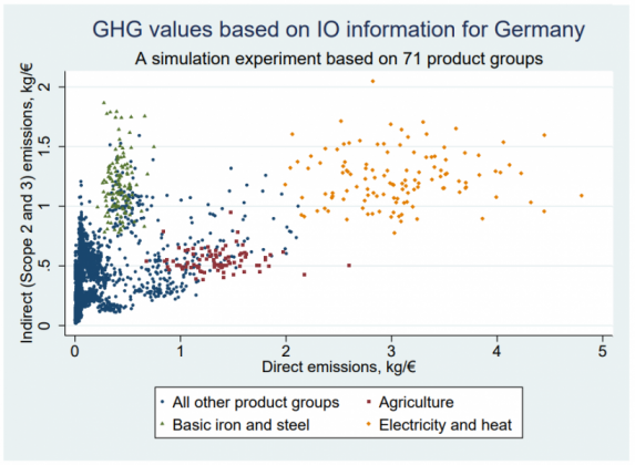
Author’s estimates and computation, based on Destatis (2021a) and Destatis (2021b).
Graph 1 displays the resulting distribution of direct emission versus indirect emission intensities. Three sectors have been singled out visually. Electricity and heat are the source of Scope 3 emissions, and they are characterised by very high direct and indirect emissions per unit of output. The GHG intensity of agriculture is also high, specifically because of CH4 (methane) due to livestock farming and NO2 (nitrous oxide) due to fertilisers. Lastly, basic iron and steel are characterised by high indirect emissions, mostly due to heavy use of products from the same sector.
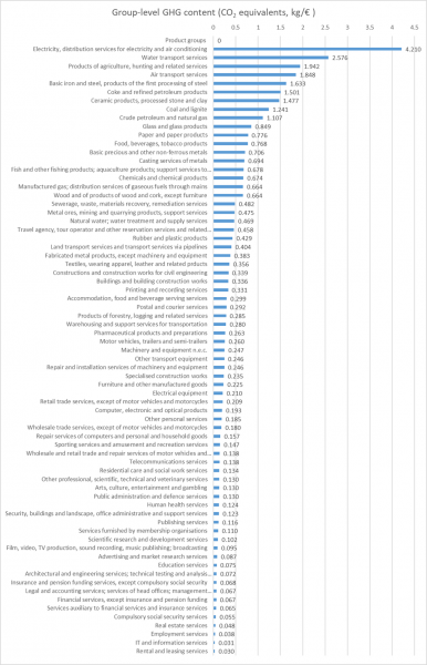
In order to get the iterations going, we need proxies as starting values. Group-level GHG contents are calculated from the IO tables and the direct emission statistics. For computations, the author uses the IO matrix for total production plus imports and the emission intensity calculated as national emissions over national production by product group. This assumes that production abroad is carried out with the same technology as national production. The shortcut is not satisfactory, but certainly more appropriate than considering only national production interlinkages in calculating GHG values. The results for sectoral GHG content are shown as a graph in Annex 2, see von Kalckreuth (2022).4
The simulation then traces the evolution of GHG value measures in a situation where each producer only knows the input coefficients of their own product and the best effort GHG value estimates of others. This can be carried out on a small and decentralised information base, and the micro-simulation allows a study of whether and how fast decentralised learning converges to the true value.
Graph 2: GHG value learning using sectoral GHG contents as initial value
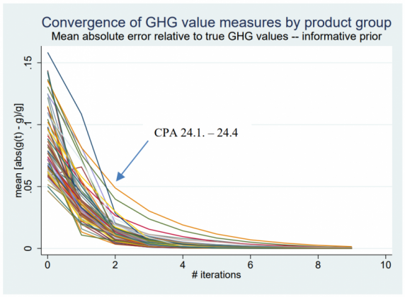
Author’s estimates and computation.
Graph 2 gives, for all product groups, a graphic representation of learning in iterations 1 to 10, depicting the mean absolute distance of estimates from the true GHG values, normalised by the level of GHG value.
Convergence is very fast for almost all products. A major exception is product group CPA 24.1.-24.4, Basic iron and steel, products of the first processing of steel, where convergence is visibly slower. This is related to a large input coefficient of 0.5 for inputs of goods of the same sector. With this, a “wrong” prior set of GHG values will be transmitted with a relatively high weight to the next iteration of the learning process.
To a certain extent, GHG value disclosure may rely on voluntary action by producers. There is a distinct commercial interest in obtaining and communicating carbon accounting information. It is also clear that some firms have good reasons to declare the GHG value of their products either incorrectly or not at all. Just as with financial costs, if there is an opportunity to make products look cheaper than they really are or to avoid talking about costs altogether, some market participants will take it.
Thus, to establish a GHG value system, some reporting obligations will be necessary. This section makes the argument that reporting obligations may not have to be broad-based. Instead, legislation only needs to make sure that a threshold volume of disclosure, e.g. from large companies, is surpassed. Under certain conditions, this will trigger a process that will end in almost universal voluntary disclosure.
If companies subscribe to an E-liability system as envisaged by Kaplan and Ramanna (2021b), it is not in their interest to conceal GHG values – if they choose not to declare their E-liability, they will not get the credit. External auditing is needed to make sure that GHG debits and credits match inventory changes. In addition, basic valuation standards need to be backed up. Producers may rig the valuation of inputs that have no GHG values attached. By distorting the accounting allocation, they can make their output look “too cheap” in terms of GHG or cross-subsidise one product line with GHG-sensitive demand by charging other product lines where demand is inelastic. Thus, as a first component, formal auditing needs to make sure that the GHG value measure is a fair estimate, using the information on direct emissions and production interlinkages existing at the company level. Auditing is carried out against disclosure standards that have to be specified in advance. It is best organised in parallel with financial auditing, with governments having the right to scrutinise dubious statements. In this respect, it is promising that the IFRS is about to change its statutes in order to set up a board on disclosing standards for environmental information.
Second, an information platform is required that makes accessible the information available on:
There is a path that leads to voluntary disclosure by (almost) all firms. Suppose that the information platform, in addition to making existing information publicly available, computes estimated average GHG content for firms of a given industry that do not disclose their E-liabilities – from the known industry averages and the known E-liabilities of the firms that do disclose. These estimates will be used to evaluate the average GHG values of inputs produced by non-disclosing firms.
Producers with low GHG values, relative to their peer group, will have a clear incentive to disclose, especially if they are active in GHG-sensitive markets. With low GHG values, they can charge higher prices to their buyers of intermediate or final goods or reap the rewards of positive publicity. This fact will generate a signal value for the decision not to disclose. The signal will be reinforced by calculating sector averages for GHG values conditional on not disclosing. With many companies disclosing, those that do not disclose will look increasingly unattractive. We may envisage an iterative process where first the cleanest firms disclose, then those that are not top tier, but still well above average, etc. In the end, the only firms to not disclose will be those with rather extreme GHG values, and the fact that they do not disclose will be informative enough.
This unravelling due to taking the average over the ever smaller number of non-disclosing companies is quite similar to the Stiglitz and Weiss (1981) account of the possible breakdown of the credit market under asymmetric information. In the scenario at hand, however, the result is a separating equilibrium with voluntary disclosure. In order to create an incentive that is great enough to trigger this mechanism on a large scale, we may need to overcome a threshold number of participating firms.
Just as in a system of market prices, information on carbon usage can be processed in a decentralised and efficient manner, even without specific disclosure obligation. The key ingredients are micro-level auditing and a centralised information platform. This is where central banks may have an important role to play. They need to collect much of the required information anyway in order to classify their assets and collateral and, in some important cases, to rate companies. In addition, they have the mandate to disseminate statistical information for policy purposes as well as all the necessary infrastructure, experience and working routines.
The following is a list of policy options for central banks resulting from the discussion above:
A limited GHG value system is conceivable, aiming at a targeted subset of products only, such as energy, transportation, agriculture and parts of the manufacturing sector; see Annex 2 for an overview. This is easier to initiate and may still reap large parts of the overall benefit. But the simplicity comes at a cost. For many input goods, GHG value coefficients will have to be imputed permanently, as even in the long run there will be no values from input providers. Good proxies would be more essential than in an encompassing GHG value system. But even in this limited version, granular information would come from producers using their private knowledge on the input composition. This is perhaps the most important feature of a system of GHG values.
The GHG value encompasses both direct and indirect GHG emissions as a consequence of the production of a good or service. Indirect emissions are the result of direct emissions in a chain – or rather a fabric – of other production processes. Those production interlinkages are key for the consistent treatment of indirect emissions. IO analysis is designed for this type of interlinkages, and in fact it has been used in tackling the issue of attributing resource consumption to final output at the sectoral level since the 1970s. IO analysis makes the structure of an interlinked system of GHG values accessible.
To fix ideas, consider the following. In production planning, every process is defined by a bill of material (BoM) that specifies all inputs, plus a route sheet that explains how to combine them. A complex production process may be decomposed into several stages. Consider the BoM of product k,
![]()
, with aki being the quantity of good i that enters the production process. There are entries for all input goods in the economy, most of them with a value of zero, of course. Let the amount of GHG emitted directly be given as dk. Let scalar gi be the GHG value of good i, the quantity of GHG that is emitted in the production of one unit. List the GHG values of all input goods in a vector as well:
![]()
The GHG value of product k is then given as the sum of direct and indirect emissions. Importantly, we do not add a definition for indirect emissions, but simply define them recursively as the GHG values of inputs:
![]()
Indirect emissions are the direct emissions at earlier stages of the value chain. The equation is both perfectly general and encompassing. It relates to products and activities and – for a defined time span – to enterprises and sectors as well.
As it stands, the equation is a definition. It helps us understand the problems associated with gathering and processing information. For actual computation, all the gi corresponding to the BoM of product k are required. If these are known, we can calculate the GHG value of product k in a straightforward way from direct emissions and the BoM. This is like computing the energy content of food: it is enough that producers know the composition of their product and the energy content of the ingredients.
If the relevant elements of g are unknown, we can use equation (1) recursively and try to compute the GHG values involved, going up the value chain from more complex intermediate inputs down to primary and primitive inputs. The structure is well known from linear production planning and IO analysis, pioneered by Wassily Leontief, and it was indeed the same author who first proposed using IO models for analysing pollution generation associated with inter-industry activity.9 Conceptually, we can solve for the GHG values of all products simultaneously. Let
![]()
be the matrix of the BoMs for all output goods, 1,…,K. With d being the column vector of the associated direct emissions, one may write:
![]()
Reordering and postmultiplying the “Leontief inverse” (I – A)-1 yields:
![]()
The GHG values of products (product k and all the others) result from their own direct emissions and the direct emissions of all the intermediate goods used for their production by intermediation of a matrix derived from the BoM that reflects the interlinkages in production. If the coefficients in the GHG equation refer to empirical production technologies actually being used to produce goods, 1,…,K, it can be taken for granted that the inverse exists and all its elements are non-negative.
As simple and beautiful as this relationship is, it is not possible to use it directly. Matrix A comprises the BoMs for all products in the economy, including those that have been imported, and if a certain input is produced using two different technologies, it should actually have two separate entries. Meanwhile, vector d collects the direct emissions that characterise all of these processes. Except for simple cases, this cannot be dealt with at the micro level. However, sector-level approximations of factor intensities using IO models are feasible. And just as the price mechanism is able to process an enormous amount of information in a decentralised way, there are ways to make the coordinated exchange of information between producers do the rest of the work.
Author’s estimates and computation, based on Destatis (2021a) and Destatis (2021b).
Destatis, Umweltökonomische Gesamtrechnungen. CO2-Gehalt der Güter der Endverwendung, Berichtszeitraum 2008-2015. Wiesbaden, 2019.
Destatis, Volkswirtschaftliche Gesamtrechnung. Input-Output Rechnung 2018 (Revision 2019, Stand: August 2020). Wiesbaden, 2021a.
Destatis, Umweltökonomische Gesamtrechnung. Anthropogene Luftemissionen, Berichtszeitraum 2000-2019. Wiesbaden, 2021b.
Hayek, Friedrich A., The Use of Knowledge in Society. The American Economic Review 35 No. 4, (1945), 519–530.
ISO (International Organization for Standardization), Greenhouse gases — Part 1: Specification with guidance at the organization level for quantification and reporting of greenhouse gas emissions and removals, ISO 14064-1:2018.
ISO (International Organization for Standardization), Greenhouse gases — Carbon footprint of products – Requirements and guidelines for quantification, ISO 14067:2018.
von Kalckreuth, Ulf, Pulling ourselves up by our bootstraps: the greenhouse gas value of products, enterprises and industries. Deutsche Bundesbank Discussion paper 23/2022.
Kaplan, Robert S. and Karthik Ramanna, How to Fix ESG Reporting. Harvard Business School Working Paper 22-005 and BSG (Blavatnik School of Government at the University of Oxford) Working Paper 2021-043, July 2021a.
Kaplan, Robert S. and Karthik Ramanna, Accounting for Climate Change. Harvard Business Review 99 (6), November–December 2021b, 120-131.
Leontief, Wassily, Input-Output Economics. New York, Oxford University Press, 1966; 2nd ed. 1986.
Leontief, Wassily, Environmental Repercussions and the Economic Structure: An Input-Output Approach. Review of Economics and Statistics 52 (1970), 262-271.
Miller, Ronald E. and Peter D. Blair, Input-Output Analysis. Foundations and Extensions. Cambridge University Press, Cambridge etc., 3rd ed. 2022.
Qayum, Abdul, Inclusion of Environmental Goods in National Income Accounting. Economic Systems Research 6 (1994), 159-169.
Stiglitz, Joseph E., and Andrew Weiss, Credit Rationing in Markets with Imperfect Information, The American Economic Review, Vol. 71, No. 3 (1981), 393-410.
Stechemesser, Kristin, and Edeltraud Guenther, Carbon accounting. A systematic literature review. Journal of Cleaner Production 36 (2012), 17-38.
WRI and WBCSD, Corporate Value Chain (Scope 3) Reporting Standard. Supplement to the GHG Protocol Corporate Accounting and Reporting Standard, 2011a.
WRI and WBCSD, Product Life Cycle Accounting and Reporting Standard: A standardized methodology to quantify and report GHG emissions associated with individual products throughout their life cycle, 2011b.
WRI and WBCSD, Technical Guidance for Calculating Scope 3 Emissions. Supplement to the Corporate Value Chain (Scope 3) Accounting and Reporting Standard, 2013.
There are other terms for the amount of GHG emitted directly and indirectly in the course of production. “GHG content” is mostly used for sectoral IO measures, while the terms “GHG footprint” and “GHG intensity” are general and not tied to any measurement framework. The term “E-liability” is a concept proposed by Kaplan and Ramanna (2021a, b) to characterise a process for collecting, processing and reporting information on GHG emissions in an accounting framework.
As part of the European Green Deal, the European Commission intends to put a carbon price on targeted imports by 2026 to avoid “carbon leakage”, i.e. the migration of industries to countries with more relaxed emissions policies. Technically, importers need to buy carbon certificates corresponding to the carbon price that would have been paid if the products had been produced in the European Union; see here official information with further links to the proposed legislation. Without a quantification of carbon content, the WTO may well consider the proposal an illegal tariff.
This is analogous to the processing of information on economic scarcity in the price mechanism, as described by Hayek (1945).
The product group-level GHG contents have been calculated here for the purposes of a simulation exercise, and they are not meant to provide statistical information. Still, as a consistency check they can be compared against the results for Germany in Destatis (2019). This publication gives a detailed evaluation of the carbon content of final use in 2008 to 2015. In spite of the differences in the reference year and some important methodological aspects, the figures compare well for the GHG content of overall production, electricity and heat and the large industrial and service sectors. For methodological differences, see von Kalckreuth (2022), fn 20 and 21.
This matches Recommendation 1 in the suggested work plan for the new G20 Data Gaps initiative.
See, in particular, WRI and WBCSD (2004) as a standard for Scope 1 and 2 emissions, WRI and WBCSD (2011a) for Scope 3 emissions at the enterprise level, WRI and WBCSD (2011b) for corresponding standards for Scope 3 emissions at the product level, and the Technical Guide on Scope 3 emissions in WRI and WBCSD (2013).
See specifically ISO 14064-1:2018 on GHG reporting at the organisation level and ISO 14067:2018 on reporting at the product level.
As already mentioned, the upcoming legislation on the carbon border adjustment mechanism and the enhancement of the scope of the carbon emissions trading systems are beneficial in this respect.
Wassily Leontief was awarded the 1973 Nobel Prize for the development of IO analysis. Leontief (1966, 1986) covers much of his work. Leontief (1970) himself introduced pollution by augmenting the technology matrix to include a row of pollution generation coefficients; see Qayum (1994) for a consistent reformulation. For IO analysis in general, see Miller and Blair (2022), and specifically Chapter 10 for environmental IO analysis.