Using pre-crisis extrapolations of GDP is likely to grossly exaggerate the output cost of the Global Financial Crisis as such trends were unsustainable. Evaluating the loss in comparison with pre-crisis trends in potential output, suggests that the median loss among OECD countries experiencing a bank crisis was still more than 6%, with this almost entirely accounted for by lower productivity, rather than lower employment. Much of the lower post-crisis productivity is in turn accounted for by lower growth in capital per worker, whereas declining tfp growth pre-dates the financial crisis.
Assessing the damage from the Global Financial Crisis (GFC) is not straightforward, even with the benefit of hindsight provided by ten years of history, because the counter-factual of what might have happened in its absence is unknowable. However, a simplistic, but commonly adopted approach of comparing the post-crisis path of GDP with the pre-crisis trend, exaggerates the cost and can lead to misleading policy conclusions. Such an approach is akin to treating the GFC as a meteorite from outer space which is completely unrelated or ‘exogenous’ to preceding macroeconomic developments. This is implausible because the pre-crisis trend in GDP involved unsustainable trends in asset prices, most obviously house prices, driven by a long period of rapid excessive credit growth across most of the advanced economies. Similarly ageing has started to dent the quantity of labour in many economies, so reducing their capacity. Hence, the counter-factual represented by the extrapolation of the past trends in GDP was never attainable.
A more plausible basis for a counter-factual is an extrapolation of pre-crisis trends of potential output, where potential output is an estimate of a sustainable measure of GDP2. The difference between these two approaches is first illustrated by considering the OECD countries as a group and using aggregated measures of potential output that are regularly published in the OECD Economic Outlook. A simple-minded extrapolation of OECD-wide GDP per capita implies an ever-widening loss, which is currently more than 10% of GDP, whereas compared to a pre-crisis extrapolation of potential output per capita implies a smaller loss of around 2-3 percentage points of GDP (Figure 1).
Figure 1. OECD GDP per capita compared with alternative pre-crisis Trends
Index 1990=100
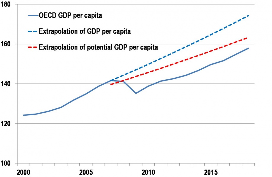
Notes: The extrapolations are based on extending the 2000-07 trends in GDP per capita and potential GDP per capita over the period 2008-18.
Source: OECD Economic Outlook June 2018 database.
However, the estimated cost of 3% of GDP for the OECD as a whole hides large variations among countries. Among the 19 OECD countries that experienced a banking crisis, following the same approach, the median loss in output is more than double that, at around 6%.
The estimates of potential output also provide an estimate of how the loss was incurred and some clues as to some policy lessons that might be drawn. Perhaps surprisingly, in nearly all OECD countries, aggregate employment rates have recovered and are close to, or have even surpassed, the pre-crisis levels, although some groups (for example young workers) have suffered more permanent losses than these aggregate calculations suggest. A notable exception is the United States, where the aggregate employment rate is still more than 3% below the pre-crisis level, which may be partly explained by the effects of opioid addiction3.
Instead, the main lasting macroeconomic damage from the GFC is accounted for by lost productivity. OECD estimates suggest that for a majority of OECD countries experiencing a banking crisis, most of this lost productivity is accounted for by lower growth in capital per worker, rather than lower total factor productivity (TFP) (Figure 2). The loss in capital per worker illustrates how a severe adverse demand shock can be transformed into an adverse supply shock via an accelerator effect on investment that then reduces the capital stock4. In addition, increasing evidence, including from firm level studies, suggests that many countries where interest rates were particularly low in the pre-crisis period, especially in Southern Europe, experienced a substantial misallocation of capital. These countries are also among those that experienced a more abrupt post-crisis adjustment in capital stock growth. The fall in capital stock growth was also exacerbated in some countries that cut back on public investment after the crisis.
Figure 2. Estimates of the loss in trend productivity due to the Global Financial Crisis
% difference in the level in 2018, relative to pre-crisis trend
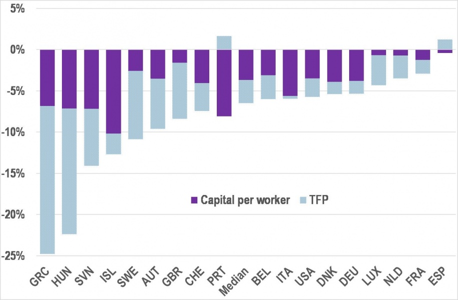
Notes: The countries shown are those OECD countries experiencing a banking crisis after the GFC. The bars show the estimated deflection in components of trend productivity relative to a pre-crisis trend distinguishing between a capital per worker component and a tfp component.
Conversely, much of the loss in tfp can be traced back to weakening trend tfp growth that pre-dates the Global Financial Crisis. This in turn would suggest that policy may be better directed to addressing more long-standing causes, such as the increasing divergence between productivity performance of frontier and laggard firms, which may be symptomatic of rising entry barriers and reduced contestability5.
***
Appendix: Methodology for evaluating the output cost of the financial crisis
The current OECD method of estimating potential output assumes a Cobb-Douglas production function, which can be simplified so that potential output (Y*) is represented in terms of potential employment (N*), the capital stock (K) and labour-augmenting technical progress (E*), so that:
(1) y* = α (n*+ e*) + (1- α) k,
where lower case letters denote logs and α is the wage share.
Potential output per head of population (P) can be explained in terms of two components: trend productivity and a potential employment rate, as follows:
(2) ∆(y*- p) = ∆(y*- n*) + ∆(n*- p).
This trend productivity component can also be split into two components to give an effect from labour efficiency (or equivalently an effect from total factor productivity) and an effect from changes in capital per worker, represented as:
(3) ∆(y*- n*) = α ∆e* + (1- α) ∆(k – n*).
For the purposes of the post-crisis counter-factual, these two components of trend productivity are extrapolated at the same average growth rate as experienced over the pre-crisis period 2000-07. The potential employment rate component (the second term in (2)) is estimated in way which adjusts for cyclical effects, and so for the purposes of the counter-factual is assumed to remain at its pre-crisis (2007) levels.
The effect of the crisis is then evaluated as the difference between the counter-factual trend described above and the latest estimates and projections of potential output consistent with the projections published in the June 2018 OECD Economic Outlook. This “crisis hit” to the level of potential output can then be decomposed into an effect on trend productivity, which can be sub-divided into effects from total factor productivity and capital per worker, and the potential employment.
The authors are both members of the OECD Economics Department. The opinions expressed and arguments employed are those of the authors and should not be reported as representing the OECD or its member countries.
The approach described here represents an update of the calculations presented in:
Ollivaud, P., and D. Turner (2015),”The effect of the global financial crisis on OECD potential output”, OECD Journal: Economic Studies, OECD Publishing, vol. 2014(1), pages 41-60.
A more in-depth analysis of post-crisis trends in employment and labour force participation in the United States, including the effect of the opioid crisis, is provided by:
OECD (2018), OECD Economic Surveys: United States 2018, OECD Publishing, Paris,
https://doi.org/10.1787/eco_surveys-usa-2018-en.
A more detailed analysis of the effect of the crisis on productivity in OECD countries, in terms of its effects on capital per worker and tfp, is provided by:
Ollivaud, P., Y. Guillemette and D. Turner (2018), “Investment as a transmission mechanism from weak demand to weak supply and the post-crisis productivity slowdown”, OECD Economics Department Working Papers, No. 1466, OECD Publishing, Paris, https://doi.org/10.1787/0c62cc26-en.
Evidence on the difference between the productivity performance of firms at the global frontier and laggard firms, as well as possible causes and policy responses, is provided by:
Andrews, D., C. Criscuolo and P. Gal (2016), “The Best versus the Rest: The Global Productivity Slowdown, Divergence across Firms and the Role of Public Policy”, OECD Productivity Working Papers, No. 5, OECD Publishing, Paris, https://doi.org/10.1787/63629cc9-en.