How does changing pricing behavior affect inflation? Evidence from Euro Area microdata

Why did we fail to predict the acceleration and persistence of inflation since early 2021? Was it because our forecasting tools relied too much on a parameterization which reflected the long non-inflationary period? This note provides some evidence from new Euro area micro data that supports this notion by showing that key time series properties of the micro level panel data did change a lot along with the acceleration of inflation, and in a way which is hardly consistent with conventional Calvo pricing schemes. Moreover, we find that there have been strong state-dependent elements in the pricing schemes suggesting that past pricing errors are compensated later on. Thus, the more there is relative price dispersion, the more there is a need for corrective action which may even lead to overshooting properties in aggregate inflation.

What went wrong?

It is hard to deny that most economists failed to anticipate the current high inflation. Not only it is true with individual economists but also most relevant institutions. Obviously, there are various seemingly good reasons for this failure including the long stretch of low inflation, the unprecedented nature of the COVID-19 pandemic, fiscal and monetary stimulus, the war in Ukraine, global supply chain disruptions, etc. But even when these factors receded, inflation continued faster than expected. Against this background, it is evident that the economic tools that economists routinely use also deserve some blame. A key tool in economic analysis is currently the New Keynesian Phillips curve where inflation expectations play the key role. Inflation expectations become instrumental because of perceived price rigidities which crucially affect pricing decisions. A standard technical solution to modelling price rigidities is the so-called Calvo-pricing scheme where it is assumed that prices can be changed only at certain points of time where the probability of a permission to change prices follows a stochastic process with a given frequency. In this setting, this frequency/probability is a “deep” parameter so that changes in the rate of inflation just reflect changes in the size of price changes. True, there has been some evidence that this setting (relative importance of intensive and extensive margin of price changes) is consistent with the data (see e.g. Klenow and Kryvtsov (2005) and Nakamura and Steinsson (2013)) but we have several reasons to suspect that at least with the current inflation the Calvo setting does not work well and that obviously has powerful policy implications (Ascari and Haber (2022)). Just recently, Dunn et al. (2023) using the UK Decision Marker Panel data showed that firms that use state-dependent pricing schemes have had clearly higher growth rates of prices compared with firms which use time-dependent pricing.

There are several reasons for this sceptic attitude. First of all, we have seen that huge changes have taken place in commodity pricing because of the IT revolution, the (menu) costs due to price changes have come down dramatically (see e.g. so-called Amazon pricing schemes; Cavallo (2022)) and the nature of costs have also changed so that the pricing of individual items has come down but not the costs that mainly come from the construction of pricing schemes (i.e. construction of tolerance levels; see e.g. Werning (2023)). Another obvious problem with pricing is the idea that the probability of price changes does not reflect in any way the economic environment of a firm. Thus, a firm, which has not changed its price and is lagging behind its competitors patiently waits for the permission to change its price. But as pointed out by e.g. Golosov and Lucas (2007), this does not make sense, and we should, instead of the Calvo scheme, adopt some form of state-dependent pricing.

Changed time-series properties

In this paper we try to open this issue by making use of novel data from Euro area which consists of 280 commodity groups (even though we here call them “commodities”). These data are monthly and cover a long period stating from the 1990s but the complete data cover only 2016M12-2023M5. Anyway, there are 21840 observations in the data. So, the data have some genuine micro data features: we can compute relative prices and cross-section moments of the data. Thus, we can abandon the assumption of a representative firm and evaluate what it means if the Calvo parameters for different commodities/firms differ.

To get some idea of the basic features of the data, particularly from the point of view of Calvo pricing, we report some basic data on actual inflation and on simulated data which follows the Calvo scheme. For this purpose we have constructed data so that the probability of price change (permission to change the price) in one month is either 0.10, 0.33 or 0.50. For simplicity, we have assumed that all price changes are positive, and of the “size” of one. Alternatively, we assume that the price changes increase in a trend-like manner where the trend is the same for all firms or alternatively that are firm-specific. Then we just the look at the autocorrelation function of the respective series and compare it with the one of actual inflation. The results are displayed in Figure 1.

The basic features of the simulated data are immediately obvious. The micro data are basically “white noise” while the actual data are not. The striking feature in the actual data is the very strong seasonality component, which suggests that prices are changed randomly but at fixed intervals (like in the Taylor staggered contracts’ two-period model) When inflation wakes up, the seasonality component becomes clearly smaller and the AR1 component somewhat stronger. This also shows up in average values (low-right corner of the table). All in all, we see that the structure of time series changes markedly in different inflation regimes.

Figure 1: Comparison of the autocorrelation structure of the simulated and actual data


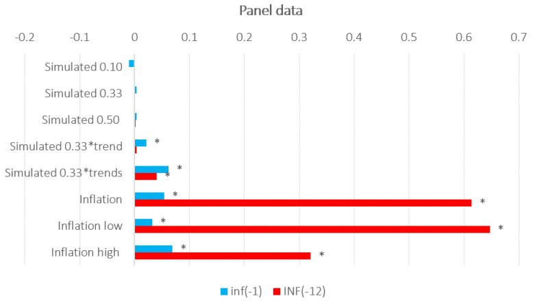
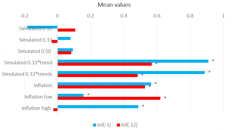
Notes: Stars indicate statistical significance at the 0.05 level. “trend” indicates a common trend instead in scaling the price change dummies. In the case of “trends” different scales are used for the trend of each price series. “simulated” 0.10” indicates simulated data with 0.10 monthly frequency, and so on. The sample period is 2017M1 2023M5. 2017M1-2021M1 (2021M2-2023M5) is the low (high) inflation period.

Simulated micro series are in all cases quite different from actual series. No surprise, that the 12-month seasonal component is missing. In order to get some autocorrelation to micro or macro series we have to assume that the size of the prize increase increases steadily in a trend-like manner. Different commodity-specific trends do not make much difference but obviously the assumption that all changes are positive is quite relevant. Seasonal autocorrelation in the size of price changes would presumably require strong seasonality on the output series.

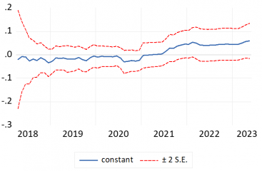
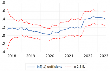
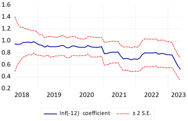
The changing role of seasonal components with the actual panel data shows up also if we estimate a simple autoregressive model in a recursive way, see Figure 2. Quite clearly, the results are similar to those in Table 1: the seasonality pattern changes dramatically when we move from low inflation to high inflation in 2021.

Figure 2: Recursive estimates from a time series model with the 1. and 12. lag on the right-hand-side

State dependent pricing

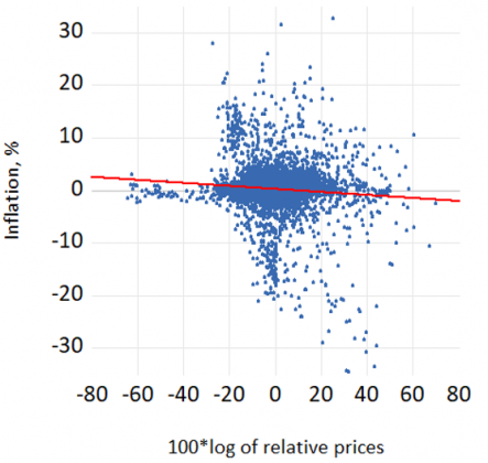
Turn now to the more important issue of state-dependent pricing. Given the novel data, the interesting question is whether current prices are affected not only by (aggregate) market condition but also the relative prices. An obvious hypothesis is that if the firm is lagging behind other firms in terms of prices (has not increased prices in the same way as competing firms), it has, ceteris paribus, an incentive to increase prices more than the other. To find out whether this is true, we estimated a set of models from the panel data so that current inflation is explained by the lagged inflation and lagged (log) relative prices (individual prices in relation to mean or median values). In addition, we had proxies for the range of prices or the standard deviation of inflation or relative prices. The latter proxies were introduced to address the idea that when inflation increases, also relative price differences increase and the volatility of inflation increases. The idea is that that should have a positive effect on inflation because more pricing errors take place and hence more price adjustments are required.

Empirical analysis suggested that is indeed the case. See Figure 3. So, we find that there is strong negative statistical association between relative prices and micro-level inflation (the association becomes much stronger when we add fixed effects and seasonality as controls). Thus, when lagging behind the average of prices, we tend to increase prices more than firms which are close to the average or above the average. Obviously, vice versa applies. The fact that also the range (or volatility) measures are clearly significant completes the story. In high inflation, the range of relative prices tends to increase and there will be more firms that need to make different price adjustments. The dominating feature is, of course, the “error-correction mechanism” with a gradual return to the “normal level” but it is obvious that the process has some potential elements of overshooting. Firms not only make necessary adjustments due to costs (such as real marginal costs) but also try to compensate earlier pricing errors. The bigger the range of relative prices (or inflation), the more firms have the compensation motive.

Figure 3: Relationship between relative prices and inflation

An interesting question is whether the adjustment is linear or nonlinear due to some specific features of menu costs. We do in fact find that this is the case. Thus, when we estimate a so-called threshold model, we find that the relative price effect is operational only when we are far away from the mean values, or when the magnitude of inflation or deflation is nontrivial (Figure 4).

Figure 4: Threshold model estimates for the coefficient of the relative price variable

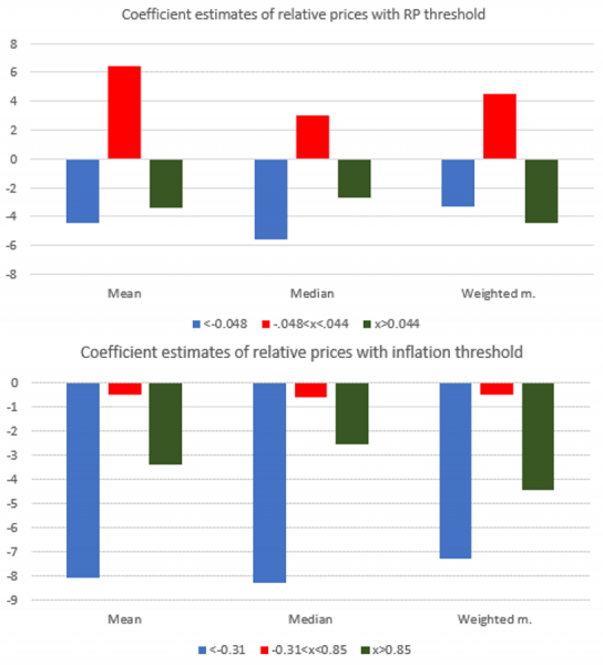
Notes: “Mean” means that individual commodity prices are compared with the unweighted mean. Median and weighted m. have an analogous interpretation. The threshold values are below the bars.

It looks like the effect is somewhat stronger with negative values of (log) relative prices indicating that firms (industries) which are lagging behind are more aggressive in adjusting prices than those above the mean values. That has an obvious interpretation: firms that are above the mean values can correct the “problem” by doing nothing because inflation takes care of the necessary adjustment. As for inflation, there also seems to be some sort of corridor in which no action is taken. Only when inflation (or deflation) is high enough, does scrutiny of the current relative price situation become worthwhile. The relative price effect is strongest when (absolute) prices have fallen in the past but slightly less strong when prices have already increased in the past.

Some policy conclusions

Our microdata suggests that we should be careful in relying on standard Phillips curve specifications which rely on the assumptions that the key parameters reflecting pricing behavior are invariant over different inflation regimes. This invariance assumption can lead to a considerable downward bias in inflation forecasts. Moreover, we should not only focus on aggregate values implicitly assuming that the differences between firms’/sectors’ pricing behavior are of trivial importance. Quite clearly, we have many different groups of firms in this respect (in addition to “normal firms”) such as Amazon type firms with fully computerized pricing systems, firms which mainly operate in seasonal manner and firms that have completely trivial menu costs. It would be surprising, if in this environment we would have some genuinely deep (constant) parameters in the respective models.