This brief is based on the paper entitled “Decomposing the monetary policy multiplier”, by the same authors. The views expressed here are those of the authors and do not necessarily represent the views of the Bank of Italy, the Federal Reserve Bank of San Francisco or the Board of Governors of the Federal Reserve System.
Why does the influence of monetary policy on economic activity change over time? And how do monetary policy decisions interact with the pricing of risk in financial markets? This policy brief shows that stock and bond prices are far more sensitive to unexpected increases than decreases in interest rates, and the extent to which markets respond (or fail to respond) to the decisions taken by the Fed has a critical influence on the subsequent behavior of inflation, output and employment. The ‘financial multiplier’ of a monetary policy shock, defined as the ratio between the cumulative responses of employment and credit spreads at the one-year horizon, is negligible for monetary expansions and large and negative for monetary restrictions, specially if these take place under strained credit market conditions.
Financial markets are known to play an important role in the transmission of monetary policy (see, e.g. Gertler and Karadi, 2015; Caldara and Herbst, 2019). Moreover, recent research has found that monetary policy affects economic outcomes differently depending on the nature of the intervention and the state of the business cycle (see, e.g. Tenreyro and Thwaites, 2016; Angrist, Jordà and Kuersteiner, 2018). In this brief we ‘join the dots’ between these findings, showing that markets respond in different ways to monetary shocks depending on the direction in which the Fed is moving and that this has important implications for the overall impact of the shocks on the real economy. On average, unexpected monetary expansions leave asset prices and output virtually unchanged, while unexpected contractions cause a sharp drop in stock and bond prices, an increase in borrowing costs for firms and households, and a protracted decline in inflation and economic activity. This mechanism is further reinforced if credit spreads are high to begin with, implying that the shock hits the economy at times of high uncertainty and tight credit conditions. In many ways, what matters for the business cycle is the actual cost of credit faced by borrowers in the economy rather than the short-term, risk-free rate maneuvered by the Fed. Hence, an appropriate calibration of the monetary stance requires a careful assessment of how financial conditions are likely to change in the medium term in response to policy interventions. To facilitate this calibration exercise, we compute ‘multipliers’ that are defined as the ratios between the real response and the financial response to a given monetary shock over a given time horizon. The multipliers provide a rough estimate of the ‘bang’ (e.g. change in employment) that the Fed can get for a given ‘buck’ (change in the market price of risk, as measured for instance by credit spreads). We find that expansions carry a multiplier that is statistically undistinguishable from zero, while restrictions have large negative multipliers that are also sensitive to financial conditions. These patterns are consistent with the idea that banks, firms and households operate close to their borrowing limits, and an unexpected increase in interest rates triggers defensive, risk-off type of reactions (in the form of asset liquidations, deleveraging and/or pairing down of investment projects) for which there is counterpart when interest rates decline. They also suggest that central banks may inadvertently over-tighten the monetary stance in times of financial uncertainty.
Investigating the asymmetries in the transmission of monetary shocks onto specific financial or macroeconomic indicators is relatively straightforward. In keeping with recent research advances in the field, we measure monetary surprises looking at changes in interest rates in narrow time windows around FOMC policy announcements,1 and estimate regression models that allow positive and negative surprises to have a different impact on the business cycle.2 The data is monthly and it covers the period 1990-2017. The results are displayed in figures 1 and 2 below. The figures show the estimated responses to a representative one standard deviation monetary surprise, which is associated to a (positive or negative) change of approximately 5 basis points in the three-month fed funds futures rate. Qualitatively, the results are very intuitive. Expansions (in blue) stimulate output, employment and prices, and cause a decline in credit spreads and the Financial Condition Index. Restrictions (in red) have the opposite effects. Quantitatively, however, the difference between expansions and contractions is stark: restrictions have a much larger and statistically more significant impact on all variables. The same is true for other financial indicators, including for instance the S&P 500 stock price index or the VIX volatility index. An interesting implication of these results is that the estimates obtained from simpler, linear models of the transmission mechanism, which implicitly mix positive and negative shocks, are mostly driven by monetary restrictions.
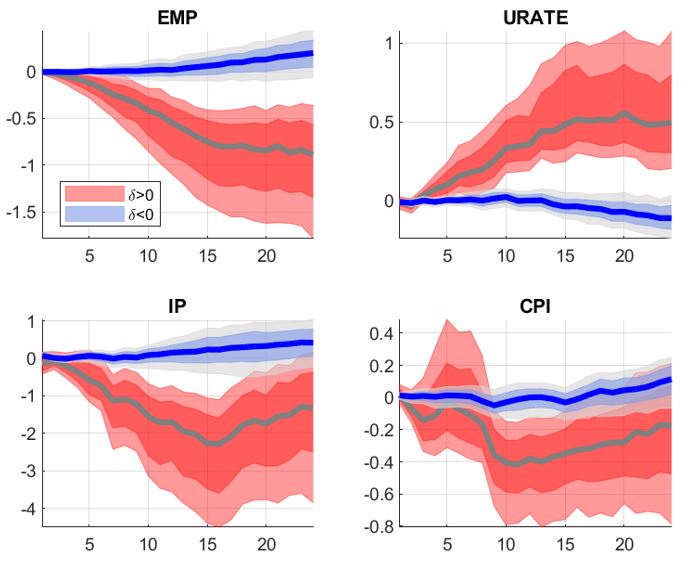
Responses of Employment, Unemployment Rate, Industrial Production and Consumer Price Index to expansionary (blue) and contractionary (red) monetary policy shocks. The shock series comes Jarocinsky and Karadi (2020). The size of the shock is normalized to 5 basis points; the responses to an expansionary shock are multiplied by minus one to facilitate the comparisons. All responses are obtained from asymmetric local projection models, controlling for two lags of the unemployment rate, IP, employment, CPI and the EBP; the bands represent 84% and 95% bootstrapped confidence intervals. The estimation sample is January 1990-December 2017.
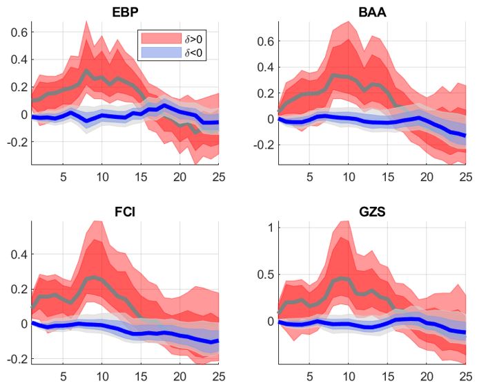
Response of asset prices to expansionary (blue) and contractionary (red) monetary policy shocks. See notes to Figure 1. The four panels report the responses of the Excess Bond Premium (Gilchrist and Zakrajsek, 2012), Moody’s BAA corporate bond spread, the Chicago Fed Financial Condition Index and the Gilchrist-Zakrajsek corporate bond Spread (GZS).
Do the asymmetries displayed in figures 1 and 2 have anything to do with one another? Establishing a link between the financial and the real side of the economy is trickier than it sounds: the data show that credit spreads and economic activity respond more to restrictive monetary shocks, but this does not necessarily mean that the real economy responds more because the spreads respond more. The double asymmetry could just be a coincidence. To rule out this possibility we switch to more articulated regression models that include an interaction between monetary shocks and the Excess Bond Premium (or some alternative financial condition indicator). The interaction term allows us to capture the possibility that the impact of the shocks on output and employment may depend on the state of financial markets.3 Based on the evidence in the previous section, we also discriminate between positive and negative interest rate surprises. Hence, the model is sufficiently articulated to account for both sign dependence (restrictions may matter more than expansions) and state dependence (restrictions and expansions may propagate differently depending on the state of financial markets). The results are summarized in figure 3. The left column shows the impact of a monetary restriction (MP+) on unemployment, industrial production and employment. For each indicator we report a range of responses obtained conditioning on different levels of the EBP: the central response assumes EBP to stay at its mean, while thicker (thinner) lines assume EBP to be above (below) the mean. The monetary tightening has a recessionary impact in all scenarios, but the magnitude of the responses hinges critically on the behavior of the bond market: the overall contraction in employment, for instance, is about -0.5% under a low EBP and -1.5% under a high EBP. The right column shows the same estimates for a monetary expansion (MP-). The impact of the expansion is generally smaller, which is consistent with the results obtained from the simpler models in the previous section, and the influence of the bond market much weaker: the employment responses lie in this case in a narrower range between zero and +0.4%. The market response to the monetary shock does matter. And it matters relatively more when investors are surprised on the upside, with interest rates that exceed expectations formed prior to the FOMC meeting.
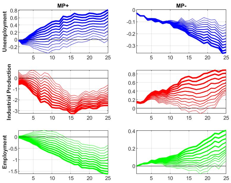
The figure shows the impact of monetary restrictions (MP+, left column) and monetary expansions (MP-, right column) on unemployment rate, industrial production and employment (rows 1, 2, 3 respectively). The shock is a positive or negative one-standard-deviation change in interest rates from Jarocinsky and Karadi (2020). For each economic indicator, the responses are obtained conditioning on different EBP levels through the Kitagawa decomposition.
The results paint a fairly complex picture of the propagation of monetary policy surprises. To summarize them, we calculate ‘multipliers’ based on the joint responses of real and financial variables to the shocks. More specifically, we define the multiplier for a given shock as the ratio between (i) the cumulative response of a real variable that enters the ‘loss function’ of the Fed (e.g. employment), and (ii) the cumulative response of a financial variable that does not enter the loss function but affects the propagation mechanism (e.g. the excess bond premium from Gilchrist and Zakrajsek, 2012). The multiplier represents the change in employment associated to a unit change in bond premium at the one-year horizon. Figure 4 shows the multipliers for employment. We again report results for the monetary tightening on the left and for the expansion on the right. To improve the readability of the chart, we calculate the ratios for only three of the scenarios considered in figure 3, focusing on the cases where EBP is one standard deviation below its mean (“loose” markets), at the sample mean (“neutral” markets), or one standard deviation above the sample mean (“tight” markets). The combined influence of sign- and state-dependence is now clear. Monetary expansions have a multiplier that is undistinguishable from zero irrespective of the level of EBP. Monetary restrictions have an average multiplier of -2: in normal times, the Fed can expect a 2% decline in employment for a 1% cumulative increase in the EBP over a one-year horizon. But the multiplier drops to zero under loose market conditions and can reach -4 when risk appetite is low.
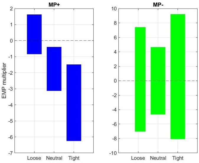
The FCM is the ratio between the Employment response and the Excess Bond Premium response at the 12-month horizon after a monetary policy surprise. The figure shows the FCMs associated to a one-standard-deviation monetary tightening (left panel) and an equally-sized monetary loosening (right panel), conditioning on three alternative financial market states (horizontal axis). Lose, neutral and tight correspond to EBP being one standard deviation below the mean, at the mean or one standard deviation above the mean. The box edges are the 16th and 84th percentiles of the bootstrapped distribution of the multipliers.
This policy brief shows that the interplay between monetary policy and financial markets is at the heart of the monetary transmission mechanism. Market investors are more sensitive to monetary contractions than to monetary expansions, and this asymmetry has important implications for the overall propagation of changes in interest rates to the real economy. Central banks need to comprehensively account for credit conditions when calibrating their monetary interventions, and face a significant risk of overplaying their hand when they raise interest rates in periods of high financial uncertainty.
Angrist, J. D., O. Jordà, and G. M. Kuersteiner (2018): “Semiparametric estimates of monetary policy effects: string theory revisited,” Journal of Business & Economic Statistics, 36(3), 371–387.
Caldara, D., and E. Herbst (2019): “Monetary Policy, Real Activity, and Credit Spreads: Evidence from Bayesian Proxy SVARs,” American Economic Journal: Macroeconomics, 11(1), 157–192.
Cloyne, J., O. Jordà, and A. M. Taylor (2020): “Decomposing the Fiscal Multiplier,” Working paper series, Federal Reserve Bank of San Francisco.
Gilchrist, S., and E. Zakrajsek (2012): “Credit Spreads and Business Cycle Fluctuations,” American Economic Review, 102(4), 1692–1720.
Gonçalves, S., A. M. Herrera, L. Kilian, and E. Pesavento (2021): “Impulse response analysis for structural dynamic models with nonlinear regressors,” Journal of Econometrics, 225(1), 107–130.
Jarocinski, M., and P. Karadi (2020): “Deconstructing monetary policy surprises—the role of information shocks,” American Economic Journal: Macroeconomics, 12(2), 1–43.
Jordà, O. (2005): “Estimation and Inference of Impulse Responses by Local Projections,” American Economic Review, 95(1), 161–182.
Miranda-Agrippino, S., and G. Ricco (2021): “The Transmission of Monetary Policy Shocks,” American Economic Journal: Macroeconomics, 13(3), 74–107.
Tenreyro, S., and G. Thwaites (2016): “Pushing on a String: US Monetary Policy Is Less Powerful in Recessions,” American Economic Journal: Macroeconomics, 8(4), 43–74.
We use the series of shocks constructed by Jarocinsky and Karadi (2020), or alternatively Miranda-Agrippino and Ricco (2021). Importantly, both account for the confounding influence of “information effects” associated to the FOMC press releases.
The regressions are local projection models (Jordà, 2005) with asymmetric terms à la Goncalves, Herrera, Kilian, and Pesavento (2021).
This extension of the LP setup allows us to perform a Kitagawa-Oaxaca-Blinder decomposition of the responses, following the strategy laid out in Cloyne, Jordà and Taylor (2020). To isolate the causal influence of financial conditions we resort to an IV strategy: monetary shocks are interacted with the fitted value of EBP obtained from a first-stage regression where we use uncertainty shocks as an exogenous driver of the spread.