A key element of the EU fiscal governance framework reform agenda is simplification. A common proposal in this context is to measure consolidation efforts only via an expenditure benchmark, thereby dropping the change in the structural balance as an operational indicator. In a recently published ECB Occasional Paper (Benalal et al. 2022), we investigate the differences between the ‘expenditure benchmark’ and the ‘change in the structural balance’. We show that the expenditure benchmark used in the EU fiscal governance framework has advantages over the change in the structural balance, on account of increased predictability and increased countercyclicality. However, it still has scope for improvement. Most importantly, we argue that taking account of interest payments in the expenditure benchmark would make fiscal policy more supportive of the monetary policy stance.
Since its inception in the mid-1990s, the EU fiscal governance framework has evolved into a highly complex surveillance mechanism. One of the complications in the current framework is that fiscal consolidation is measured and evaluated both via an expenditure benchmark (EB) and via the change in the structural balance (dSB)2. Policymakers broadly agree that a reformed and simplified EU fiscal governance framework should only rely on an expenditure benchmark.
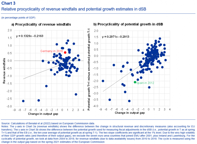
While the EB and dSB can be shown to be conceptually equivalent, they are different in the practice of the EU fiscal governance framework. These differences are explained in detail in our paper and summarised in Table 1.
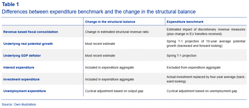
The differences in the calculation of the EB and dSB in the EU fiscal governance framework led to divergent assessments of consolidation efforts in countries. Chart 1 shows the quantitative difference between the two indicators for the euro area aggregate as well as for Germany, Italy and Spain. These three countries are of particular interest not only because of their large share in euro area GDP, but also due to the sizeable differences between the EB and dSB. Calculations show that ex post, in Germany the dSB suggests more fiscal consolidation (or less fiscal expansion) than the EB (dark blue squares). In most years, the opposite was true in Italy and Spain.
Differences between the two indicators result mainly from the accounting of revenue windfalls and shortfalls and the measurement of potential output. First, revenue windfalls and shortfalls are defined as changes in revenue which can neither be explained by discretionary measures nor by the expected stylized impact of the economic cycle.3 As the EB measures revenue-based fiscal adjustments via the estimated impact of discretionary measures, such windfalls or shortfalls only impact the dSB. There were revenue windfalls in Germany over almost the entire period observed (partly due to very strong growth in corporate tax revenue), while Italy and Spain mostly had shortfalls (purple bars in chart 1). Second, the most recent estimates of potential output are used for the dSB, while the underlying potential growth used for the EB is smoothed and frozen (fixed ex ante) before the respective fiscal year has started. In Italy and Spain, the potential growth used in the EB tended to be higher than in the dSB, which was both due to downward ex post revisions to the GDP deflator (orange bars) and to differences in real potential (green bars). Again, the opposite is true for Germany. For Germany, interest payments dropped sizeably over the whole horizon (yellow bars), again making the adjustment based on the dSB larger than the EB.4
These differences have real policy implications. For Spain, the European Commission (2013) found sizeable revenue shortfalls in its evaluation of Spain’s consolidation efforts in 2012 (which would have fallen short substantially when looking only at dSB). For Italy, the European Commission (2015) stressed the sizeable downward revisions of GDP deflators and real potential growth in its analysis of Italy’s consolidation requirements under the SGP’s debt benchmark in 2014/15. In the case of Germany, the level of the structural balance was assessed to be above the Medium-Term Objective from 2012 onwards, leading to encouragements to take a more expansive fiscal policy stance (e.g., in European Commission, 2017). However, the EB suggested a fiscal loosening of about 0.3 percentage points per year (while the debt ratio was still above 60%, except for 2019), which might have led to different policy recommendations when completely ignoring developments in the structural balance.
In view of the differences between dSB and EB, a parallel use of the indicators risks inconsistent policy messages. But which of the two indicators should be dropped in the context of a simplification of the EU governance framework?
2.1 The expenditure benchmark is more predictable than the change in the structural balance
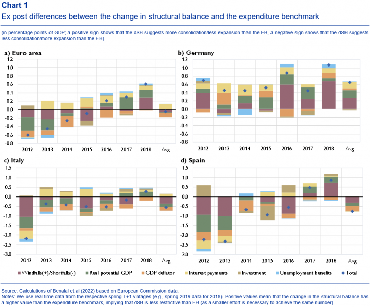
The expenditure benchmark is more predictable than the change in the structural balance by construction. First, revisions to potential growth only affect the dSB, but not the EB. When assessing the change in the structural balance, the European Commission uses the most recent (ex post) estimate of the change in the output gap, that is, GDP growth respective to potential output. Chart 2 shows that between 2004 and 2018, revisions to real potential growth rates were relatively sizeable (blue bars show the root mean squared error of revisions), implying that the part of fiscal developments attributed to the economic cycle has been revised, too.5 The EB avoids such frequent revisions as the potential GDP growth rate used to assess the appropriateness of expenditure growth is fixed ex ante for the EB.
Second, revisions in the GDP deflators further reduce the predictability of the dSB. Chart 2 shows sizeable revisions to the projections of GDP deflators (yellow bars). This contributes to revisions to nominal potential growth (orange dots) being much larger than revisions to real potential growth. This is highly relevant, as underlying potential growth rates rely on the actual deflator in the dSB. Again, this problem is avoided for the case of the EB, where projected deflators are used.
Third, the predictability of the EB is also supported by relying on discretionary revenue measures for measuring revenue-based adjustments.6 The dSB relies on the change in the structural revenue ratio, which can be affected by unexplained over- or underperformances in tax revenue. For example, in most of the occasions of large revenue windfalls in Germany and of revenue shortfalls in Spain and Italy, at least the extent of this phenomenon has come unexpected.
2.2 The expenditure benchmark is more countercyclical than the change in the structural balance
We find that the EB is more countercyclical than the dSB. A first indication can be found in Chart 1. For the euro area, this chart shows that the dSB was more stringent, measuring less consolidation/more expansion than the EB for 2012 and 2013, when real GDP stagnated, and the output gap turned more negative. This implies that countries should have consolidated more according to the dSB than when their fiscal performance had been assessed with the EB. Vice versa, dSB was less stringent, measuring more consolidation/less fiscal expansion than EB for 2016 to 2018, a time when real GDP grew above its estimated trend.
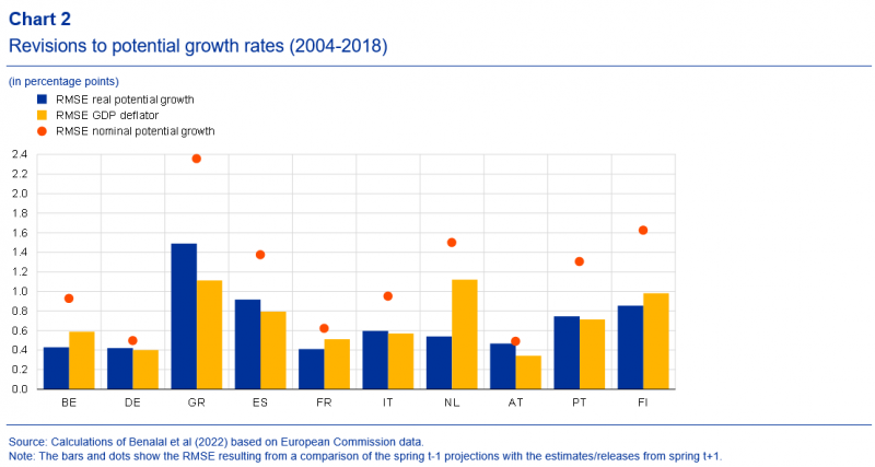
Chart 3 confirms this observation. The different definitions of both underlying potential growth7 and revenue-based fiscal adjustments tend to make the dSB less countercyclical than the EB. In economically bad times (as indicated by a decrease in the output gap; x-axis in chart 3), there tend to be more revenue shortfalls (Chart 3a) and the real potential growth rates used in dSB tend to be lower than the ones in EB (e.g., in Spain in 2012; Chart 3b). On average, a one percentage point smaller change in the output gap (i.e., GDP growth one percentage point lower for given potential growth) is associated with dSB decreasing by almost 0.3pp for a given EB.8
During the 2010s governments’ interest payments dropped substantially (as indicated by chart 1), also spurred by monetary policy actions. Monetary policy reacted with determination to persistently low inflation. This contributed to a strong decline in overall interest payments between 2013 and 2018 in the euro area. Interest expenditures of governments fell by about 0.1 to 0.2 percentage points per year from 2013 to 2018.9
Interest payments were excluded from the EB on account of the argument that they fall outside the control of governments in the short term (European Commission, 2012). However, there are good arguments for including interest payments. First, structurally lower interest rates imply the debt-to-GDP ratio can be stabilised at a lower primary budget balance, leaving more room for increases in primary expenditure (or cuts in revenue). Second, one of the main transmission channels of monetary policy is that lower interest rates induce the non-financial sectors to increase spending. A similar mechanism holds for the government sector. Lower interest payments loosen the government budget constraint. A more expansionary fiscal policy can then complement the monetary impulse.
As this argument is symmetric, i.e., fiscal space would be reduced by restrictive monetary policy (resp. higher interest rates), the inclusion of interest payments would make monetary policy more effective without endangering fiscal sustainability.
Benalal, Nicholai & Freier, Maximilian & Melyn, Wim & Van Parys, Stefan & Reiss, Lukas (2022), Towards a single fiscal performance indicator, Occasional Paper Series 288, European Central Bank.
European Commission (2012), Public Finances in EMU 2012, European Economy 4/2012, Brussels.
European Commission (2013), Analysis by the Commission services of the budgetary situation in Spain following the adoption of the COUNCIL RECOMMENDATION to Spain of 10 July 2012 with a view to bringing an end to the situation of an excessive government deficit. Accompanying the document Recommendation for a COUNCIL RECOMMENDATION with a view to bringing an end to the situation of an excessive government deficit in Spain, Commission staff working document, Brussels, May.
European Commission (2015), REPORT FROM THE COMMISSION. Italy. Report prepared in accordance with Article 126(3) of the Treaty, Brussels, February.
European Commission (2017), Country Report Germany 2017 Including an In-Depth Review on the prevention and correction of macroeconomic imbalances, SWD(2017) 71, Brussels, February.
The views expressed are those of the authors and do not necessarily reflect those of the ECB, the NBB or the OeNB.
One further complication is that the expenditure benchmark used in the preventive arm of the SGP is different from the one in the corrective arm. The calculations in our paper use the definition from the preventive arm.
The European Commission method assumes that – in the absence of discretionary revenue measures – the revenue ratio stays broadly constant over the business cycle, i.e., that revenue grows in line with GDP. Revenue windfalls resp. shortfalls are deviations from this pattern, which in the past were often due to developments in corporate taxes (e.g., the strong overperformance in Germany in the 2010s) or taxes on property (e.g., the strong overperformance in Spain in the mid-2000s, followed by a strong underperformance).
Over time, both the differences in the calculation of cyclically adjusted unemployment benefits and the smoothing of investment (esp. for larger countries) play a rather limited role. However, the large investment cuts in Spain up to 2012 and the temporary upward spike in 2015 led to temporary sizeable differences between EB and dSB in that country.
A RMSE of real potential growth rates of one-half of a percentage point (i.e., the approximate RMSE for the countries with the most stable estimates) translates mechanically into a one-quarter of a percentage point revision to the change in the structural budget balance (assuming a budgetary semi-elasticity of about 0.5).
However, some discretionary revenue measures, like changes to the tax base (e.g., closing loopholes in corporate taxation) or measures against tax fraud are very difficult to quantify, even ex post. This makes increased transparency in reporting these measures very important, e.g., one could consider publishing a breakdown in a database. Our paper also lays down some measurement problems in the current EB, most of which might be attenuated by deducting elements of non-tax revenue (especially “sales”) from the expenditure aggregate and by accounting for the impact of non-indexation of tax brackets.
This is particularly due to the freezing of spring T-1 projections for the EB as there is a tendency of macroeconomic projections to be smoother than reality (i.e., the tendency of T+1 and T+2 projections to overpredict GDP growth in recessions and underpredict it in booms).
Assuming a budgetary semi-elasticity of around one-half, the slopes in Charts 3a and 3b translate a 1 pp lower change in the output gap into a decrease in dSB by 0.134 + 1/2 * 0.297 ~ 0.28 pp compared to EB.
This shows that despite the long average maturity of public debt in most euro area Member States, the series of unconventional measures undertaken by the Eurosystem starting in mid-2012 impacted the change in interest payments both quickly and relatively strongly.