Integrated policy frameworks: The constraints of policy horizons and adjustment frequencies

The implementation lag depends on decision-making processes, which in turn reflect a mix of technical, institutional and political economy factors. As such, the lag varies across instruments. For example, the decision-making process may take longer if it involves multiple agencies rather than just one institution. Similarly, instruments that are perceived to have a strong redistributive impact raise issues of legitimacy and may require endorsement by the government or the legislature; those that involve costly modifications to business practices may also call for lengthy phase-in periods.

The adjustment frequency of instruments

The second key temporal dimension is the adjustment frequency of instruments. This reflects two factors.

The first is the same as for the policy horizon – the underlying cyclical properties of the economic variables of interest. This affects the speed with which the relevant information unfolds and hence the time span of data required for a substantive assessment. For example, it makes little sense to, say, adjust loan-to-value ratios within an interval of one quarter if no new information has emerged (unless this is part of a pre-announced plan).

The second factor is reputational costs. These reflect concerns that the reversal of policy decisions, especially if abrupt, may be perceived as a mistake and undermine credibility. This is especially so if reversals amplify rather than moderate market volatility. Such concerns increase the likelihood that policymakers make successive instrument adjustments in the same direction. But they may also reduce the adjustment frequency close to turning points: policymakers may be more hesitant to adjust the tool for fear of having to reverse the decision soon afterwards.

Policy horizons and instrument adjustment frequency: policy domains

Prevailing policy decision-making frameworks and processes reflect how the factors outlined above influence the policy horizon and the frequency of instrument adjustments. Table 1 provides a stylised summary, with horizons and adjustment frequencies defined in qualitative terms.



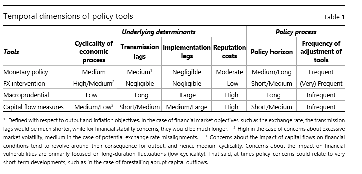
Monetary policy focuses on inflation and on closely associated output fluctuations. The cyclicality of these variables is conventionally measured by cycles of up to eight years or so (“medium cyclicality” in the Table) – typically referred to as “business cycle frequencies”. Transmission lags on financial conditions are negligible; they are somewhat longer and variable on expenditures but still consistent with the objectives. Given negligible implementation lags, monetary tools can be adjusted flexibly. The policy horizon is squarely medium-term, with a possibly longer time frame when the impact of more drawn-out fluctuations, such as financial cycles, is taken into consideration. Policy adjustments take place at regular and frequent intervals, but may also be made on an ad hoc basis in response to evolving circumstances.

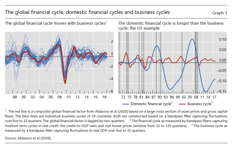
For FX intervention, policy-relevant fluctuations in exchange rates can occur at both high and medium cyclicality. Excessive exchange rate volatility, driven by self-reinforcing market dynamics, can often pose a concern in the short term; potential misalignments can become worrisome over the medium term. Concerns at medium cyclicality may relate to the impact of the exchange rate on competitiveness (the trade channel) or on domestic financial conditions (the financial channel).4 Indeed, empirical evidence indicates that the more relevant fluctuations of global financial conditions (the “global financial cycle”) operate at similar cyclicality as traditional business cycles – the left-hand panel of Graph 1 shows that measures of the global financial cycle tend to move in lockstep with those of business cycles.5 Thus, the policy horizon can vary between short and medium length, depending on the nature of the concern. The tool is quite flexible, as it involves negligible implementation lags and little reputational cost associated with reversals, given how quickly market conditions can change. When used to build up macroeconomic resilience, it has a quasi-macroprudential character, without sharing the adjustment costs of those tools.

Macroprudential measures typically have a policy horizon that is even longer than that of monetary policy measures targeted to inflation and output. The bulk of interventions address financial vulnerabilities linked to fluctuations in credit and asset prices, most notably real estate prices – the “domestic financial cycle”. Empirical evidence indicates that the fluctuations giving rise to major episodes of financial instability and large macroeconomic costs have a longer duration than business cycle ones, within a typical range of between 14 and 20 years (“low” cyclicality in Table 1). The right-hand panel of Graph 1 illustrates this for the case of the United States (Drehmann et al (2012)). Transmission lags are roughly equivalent to those for monetary policy tools – in fact, they may overlap (eg reserve requirements) and impinge on similar variables, ie those capturing financial conditions. Implementation lags, however, tend to be much longer. Given their regulatory-like character, policy decisions call for adjustments to business practices and have a potentially large impact on specific economic segments. This raises also reputational costs. As a result, not only is the policy horizon very long, but instrument adjustments are few and far-between. Indeed, Borio et al (2021) document that across a sample of 56 advanced and emerging market economies between 1995 and 2000, the average number of macroprudential measures implemented was only one per year.

Capital flow management measures share many of the features of macroprudential tools. As regulatory instruments, they tend to involve long implementation lags. The lags can be shorter with respect to adjustments to existing measures or when targeting sudden market dislocations. Transmission lags are also similar to those of macroprudential measures, although the impact of some capital flow measures can be abrupt if they unsettle investors. The policy horizon can vary, depending on whether the primary concern is the impact of capital flows on shorter-term financial conditions, and hence business cycle fluctuations, or on longer-term financial vulnerabilities. In some cases, the measures can also be oriented towards higher-frequency developments, for example to stem sudden capital flight.

Implications for integration

Reflecting the features highlighted above, the policy horizon and frequency of policy adjustments have important implications for the extent to which synergies across instruments can be realised. Differences in policy horizons limit the economic trade-offs considered in formulating policy; differences in the frequency of instrument adjustments limit the degree to which policies can respond to one another. As a result, the extent to which interdependencies are taken into account differs across tools, with implications for the overall degree and shape of policy integration.

Macroprudential policy can be regarded as a kind of fixed point. Its necessarily long horizon, determined by the objective, coupled with the inflexibility of the instruments, means that other policies will tend to take it as given.6 Macroprudential policy can react to the other policies, but these will be regarded as simply operating in the background, as their influence on financial stability takes a long time to play itself out. To be sure, there may be a temptation to use macroprudential policy more actively for business cycle stabilisation purposes. But, not unlike fiscal policy, the set of available instruments is ill suited for this purpose. Moreover, bending the policy to pursue this objective could distract it from the slower-moving build-up of vulnerabilities, which have their own dynamics, thereby impairing its efficacy.

Capital flow management measures raise similar issues. One the one hand, they may have an even more structural character, as when they are set in order to influence the overall environment of capital flows. On the other hand, they may need to be adjusted on a more ad hoc basis when addressing abrupt or intense capital flow waves. Thus, while authorities can use them as a macro-stabilisation tool, more often than not they will tend to do so sparingly. Adjustment costs and unpredictable responses naturally invite such a strategy. That said, for countries with established precedents and implementation systems, capital flow measures may be utilised more readily.

Monetary policy is best placed to internalise the other policies. This is primarily because of the flexibility of the tools at its disposal. And while the policy is overwhelmingly used for inflation and macro-stabilisation at business cycle frequencies, it could also take into consideration the slower-moving, longer-horizon developments that underlie financial stability concerns. Put differently, operationally it could place a higher weight on longer-duration GDP fluctuations, beyond the standard time spans.7

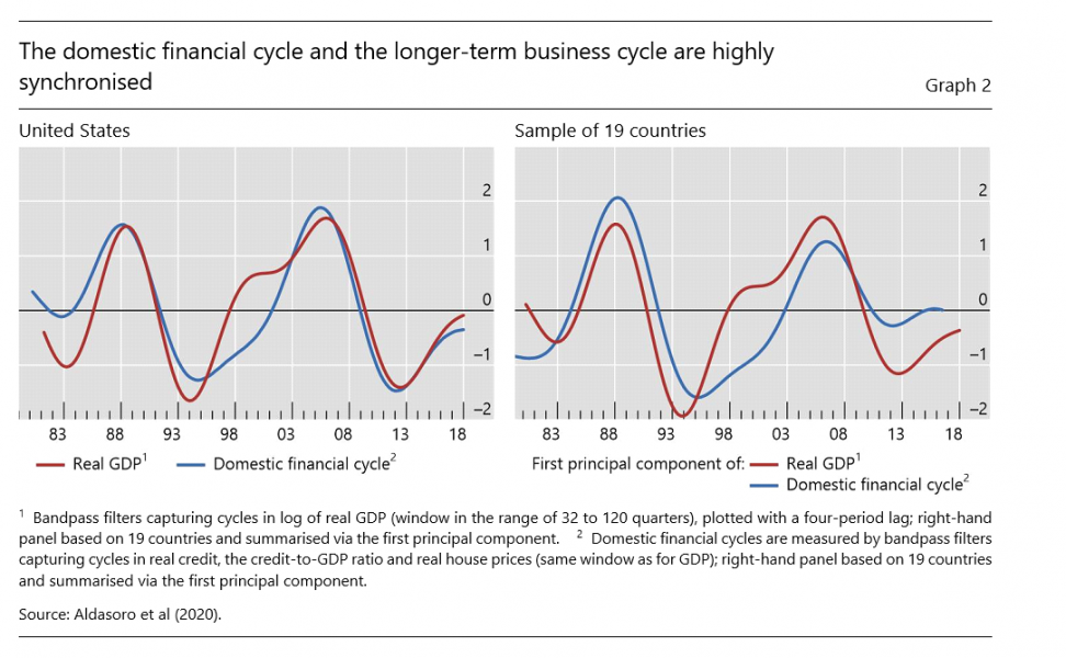
Such a longer horizon, more attentive to drawn-out output fluctuations, is important. While little appreciated, it would be consistent with empirical evidence indicating that these fluctuations tend to coincide with those of the domestic financial cycle and account for the larger share of the overall GDP variance (Aldasoro et al (2020)). For example, Graph 2 shows the remarkably close synchronisation between the domestic financial cycle and longer-term output cycles in the case of the United States (left-hand panel) – a stylised fact that applies more generally across countries (right-hand panel; for details see Aldasoro et al (2020)). As a kind of “residual policy”, the downside is that monetary policy may end up taking a larger burden of internalising the cross-instrument interdependencies. Thus, it may well have to compensate for other policies if they do not gain sufficient traction or are under-utilised. The reliance on monetary policy to support growth post-Great Financial Crisis is a case in point.


These considerations lose some of their relevance in crisis times, in which integration and synchronisation become easier. During such episodes, the active deployment of all instruments, generally operating in the same direction, becomes more natural. Synchronisation is simpler and active coordination more likely. The experience during the Covid-19 crisis is a good example.

Viewed from this perspective, formal analytical models of policy integration are subject to two limitations: (i) they have difficulties capturing the relevance of different horizons; and (ii) they generally treat all instruments uniformly. As a result, they tend to overestimate the degree of feasible integration – or at least to misinterpret its character. And they can provide a misleading picture of the desirable weights to be assigned to the different policies in pursuing a given set of objectives.

The difficulty in modelling horizons reflects two factors.

For one, it is standard for the models to assume that the horizon is infinite. This is so either explicitly, in the case of optimal policy, or implicitly, in the case of instrument rules (in the sense that the model solution and hence policy settings incorporate all information about the future evolution of the economy). In such a framework, the real-life practice of adopting different horizons is not meaningful.

In addition, most models do not distinguish between the underlying cyclicality of the relevant economic phenomena. In typical dynamic stochastic general equilibrium approaches – characterised by shock/propagation/return-to-steady-state – the shocks and their impact may affect persistence. But the models do not capture the endogenous cycles of different durations that are so important in practice. This is especially relevant for the distinction between financial and business cycles, which has a first-order influence on arrangements.

The uniform treatment of instruments further underestimates integration challenges. In the models, integration means joint calibration of tools, with all instruments adjusted simultaneously. This is so regardless of whether their path traces optimal policy or reaction functions. In practice, asynchronous adjustment is the norm and, in many cases, it could not be otherwise, given irreducible implementation lags. While, in and of itself, this need not be a major issue, it becomes more significant once it is recognised that some instruments are simply ill suited for some objectives, owing to the different cyclicality of the underlying economic processes. An important example, noted above, is assigning a role in macro-stabilisation at standard horizons to rather inflexible macroprudential tools.

Finally, the models underestimate the importance of governance arrangements. Some aspects are well appreciated. The key one is the political economy factors that may favour assigning different objectives to different authorities. This would obviously reduce the scope for policy integration. But even in the case where the central bank takes sole responsibility for the objectives under discussion, as many already do, important obstacles remain.

One common but neglected obstacle is precisely the absence of a single model of the economy on which policymakers can agree. Since no single model is able to capture the relevant elements of the workings of the economy, different central bank departments come with their very different perspectives, rather than the unified one needed to best exploit potential synergies. For instance, macroeconomic departments in charge of informing monetary policy tend to focus on aggregate developments, often seen through the lens of stylised structural models that rule out endogenous financial cycles and instability. By contrast, financial stability departments consider such cycles important, place much more emphasis on detailed sectoral developments and rely for the most part on reduced-form techniques. Bridging the different perspectives is difficult, and it is left to the policy decision-making level to reconcile them. So far, this has proved very hard.

Conclusion

The scope and effectiveness of policy integration rests on key features of the policy decision-making process. This note has highlighted how the temporal dimensions of this process affect the extent to which synergies across policy instruments are, or can feasibly be, taken into account in practice. Neglecting these factors can lead to inappropriate or impractical assignment of weights to the various policies in the pursuit of a given set of objectives.

What is the scope for improvement in the practice of integration? The most critical, often neglected, element is probably the treatment of the policy horizon. The horizon largely dictates what does and does not fall in the purview of policymakers charged with controlling a particular set of instruments.

The key challenge is for policies to take into consideration their influence on economic developments beyond their immediate operational horizon. Specifically, for instruments that are amenable to adjusting flexibly in response to short- and medium-term fluctuations, making sure that their policy horizon does not become too short could help promote complementarities across instruments.

The potential gains apply, in particular, to FX intervention and monetary policy. This is precisely because they can flexibly accommodate a range of horizons. Here, consistency in the deployment of the tools is key. In the case of FX intervention, day-to-day operational objectives – such as targets around technical support levels for the exchange rate – should remain sufficiently anchored to high-level monetary policy objectives. For monetary policy, taking into consideration its impact on longer-term macroeconomic stability through its influence on the domestic financial cycle should help to take some of the load off macroprudential policy. In both cases, adjustments to institutional setups matter. They would involve adjustments to the make-up of policy committees, to the types of policy inputs as well as to analytical frameworks. The adjustments would help better capture the relevant trade-offs, which are often intertemporal in nature.

References
Age nor, P and L Pereira da Silva (2021): “Macroeconomic policy under a managed float: a simple integrated framework”, mimeo.

Aldasoro, I, S Avdjiev, C Borio and P Disyatat (2020): “Global and domestic financial cycles: variations on a theme”, BIS Working Papers, no 864.

Bank for International Settlements (2019): “Monetary policy frameworks in EMEs: inflation targeting, the exchange rate and financial stability”, Annual Economic Report 2019, Chapter II, June.
——— (2020): Capital flows, exchange rates and policy frameworks in emerging Asia, a report by a Working Group established by the Asian Consultative Council of the Bank for International Settlements, 27 November.

——— (2021): Capital flows, exchange rates and monetary policy frameworks in Latin American and other economies, a report by a group of central banks including members of the Consultative Council for the Americas and the central banks of South Africa and Turkey, 15 April.

Borio, C (2018): “Macroprudential frameworks: experience, prospects and a way forward”, speech at the BIS Annual General Meeting, Basel, 24 June.

Borio, C, I Shim and H S Shin (2021): “Macro-financial stability frameworks: experiences and challenges,” mimeo.

Cerutti, E, S Claessens and A Rose (2019): “How important is the global financial cycle? Evidence from capital flows”, IMF Economic Review, vol 67, pp 24–60.

Comin, D and M Gertler (2006): “Medium-term business cycles”, American Economic Review, no 96, pp 523–51.

Drehmann, M, C Borio and K Tsatsaronis (2012): “Characterising the financial cycle: don’t lose sight of the medium term!”, BIS Working Papers, no 380, June.

Hofmann, B, Ilhyock S and H S Shin (2020): “Bond risk premia and the exchange rate”, BIS Working Papers, no 775, April.

International Monetary Fund (2020): “Toward an integrated policy framework”, IMF Policy Paper, October.

Rey, H (2013): “Dilemma not trilemma: the global financial cycle and monetary policy independence”, paper presented at the Federal Reserve of Kansas City Economic Policy Symposium “Global dimensions of unconventional monetary policy”, Jackson Hole, 22–24 August.